
DAML [KDD’19] review
Abstract
DAML(dual attention mutual learning)의 모델 설명은 크게 2 부분으로 나뉜다.
we utilize local and mutual attention of the convolutional neural network to jointly learn the features of reviews to enhance the interpretability of the proposed DAML model
Then the rating features and review features are integrated into a unified neural network model, and the higher-order nonlinear interaction of features are realized by the neural factorization machines to complete the final rating prediction.
즉, 첫번째로, 모델의 interpretability 를 높이기 위해 CNN의 input으로 들어가기전 word 단계에서의 local attention과 CNN 단계에서 convolution 연산시 user와 item의 연관성을 고려하여 feature 단계에서의 mutual attention을 사용하여 user에 대한 latent factor vector와 item에 대한 latent factor vector를 구하였다.
또한, rating 을 추정할때 item과 user간의 복잡한 관계에 의한 계산을 위해 unified neural network구조를 이용하였다.
Introduce
여기서는 이 논문의 모델에 대한 이유를 convention과 비교하여 설명한다.
일단 Matrix Factorization 방법은 user와 item사이의 관계를 나타내는 records를 이용하여 user의 preference 와 item의 attribute를 뜻하는 latent factor vector를 찾는 것이다.
단순히 rating을 이용하여 rating를 prediction하는 방식은 왜 유저가 이 item에 대해 rating 을 이렇게 했는가에 대한 설명없는 user, item, rating 정보만을 이용했으므로 추정한 rating 값들을 얻더라도 unexplained recommendation이며 cold start problem을 가지고 있다.
따라서, 이 논문에서는 user 의 preference 와 item의 attribute 정보가 풍부한 review를 이용한 방식에 집중하였다. 단순히 review를 Bag of Words 로 처리하여 Neural Net에 이용하는 것보다는 review에서 문맥을 고려한 feature 추출을 효과적으로 하기위해 CNN 구조를 사용하였다.
논문에서 conventional 한 방식들에 대한 소개와 한계점에 대해 요약하였다.
the review text of users and items usually contains semantic information related to users and items, without considering the relevance of features between them. It may lead to great deviation to predict users’ preferences
기존의 user와 item 의 latent feature 를 얻는 방식은 user와 item에서 각각 따로 latent feature 를 구하였다. 이렇게 하면 user와 item 사이의 semantic 정보를 고려하지 않게 된다. 예를 들면, 어떤 유저가 시계에 대해 어떤 특성을 좋아해서(시계의 디자인이 동그란 모양이라던지) review와 rating에 그런 상관 관계에 대한 정보가 녹아 들어 간 상황을 생각 할 수 있다. 그렇게 feature 사이의 mutual 한 관계를 고려하지 않는다면, user의 preference를 예측하는데 deviation이 클 것이라는 것이 이 논문의 주장이다.
There are two kinds of fusion methods. One is the traditional data fusion method based on MF or Factorization Machines (FMs). However, this method fails to capture the complexity between features in different modalities
또한, user와 item의 feature 를 이용하여 rating을 prediction 하는것은 MF, FM 방식 2가지 였다. 하지만 이 두 방법들은 feature들 사이의 복잡한 관계를 capture하지 못한다는 한계가 있다.
The other is a straightforward one that treats features extracted from different data sources equally, concatenating them sequentially into a feature vector for recommendation tasks. Nevertheless, simply a vector concatenation does not account for any interactions between latent features, which is insufficient for modelling the collaborative filtering effect
다른 방식으로는 external data source 를 이용하여 feature vector를 구한후에 그 feature 를 concatenation하추천 시스템에 이용하는 것이다. 하지만, 단순히 concatenation하는 것은 latent feature들 간의 상호작용을 설명하지 못하며, collaborate filtering 효과에 대해 불충분한 방식이다.
Architecture
모델은 Feature Learning Module과 Feature Interaction Module 2 부분으로 나뉜다.
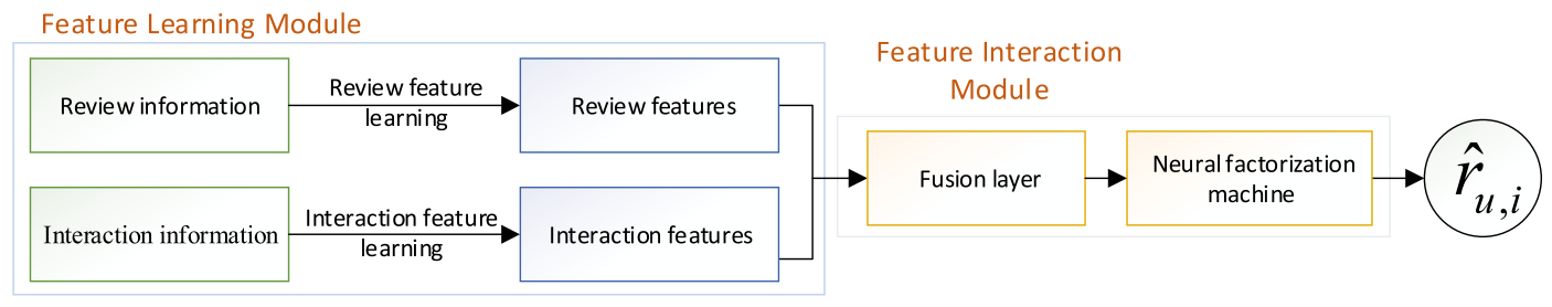
Feature Learning Module은 Local attention과 Mutual attention 2가지의 attention 방식을 취하고 있다.
ProPosed Model
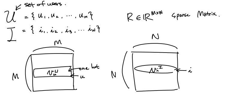
Problem Formulation
\(\begin{aligned} \mbox{Inputs: } \\ & \mbox{set of users} ~~ \mathcal{U} = { \{u_1,u_2, ..., u_M \} } \\ & \mbox{set of items} ~~ \mathcal{I} = { \{i_1,i_2, ..., i_M \} } \\ & \mbox{set of set of words by users X} = { \{x_1,x_2, ..., x_M \} } \\ & \mbox{set of set of words for items Y} = { \{s_1,s_2, ..., s_N \} } \\ & \mbox{explicit ratings} ~~ \mathbb{R}^{M \times N} \ni R \ni r_{u,i} \in \mathbb{R}\\ \end{aligned}\)
어떤 user $u$ ,item $i$ 에 대한 onehot vector
 \(\begin{aligned}
\mbox{output:} \\
& \mbox{for any user} ~ u, ~~~ \hat{r}_{u,i}\\
& \mbox{based on} ~~ f_u: v_u^U, v_i^I, x_u, s_i \rightarrow \hat{r}_{u,i}
\end{aligned}\)
\(\begin{aligned}
\mbox{output:} \\
& \mbox{for any user} ~ u, ~~~ \hat{r}_{u,i}\\
& \mbox{based on} ~~ f_u: v_u^U, v_i^I, x_u, s_i \rightarrow \hat{r}_{u,i}
\end{aligned}\)
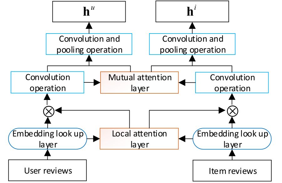
Feature Learning Module
Embedding lookup layer
user $u$ , item $i$ 에 대한 review에 쓰인 단어들의 embedding된 벡터를 lookup 하는 과정이다.
user의 관점과 item이 동일하기 때문에
어떤 user $u$ 에 대해 review에서 쓰인 단어들에 대한 embedding vector들을 look up 을 설명할 것이다.
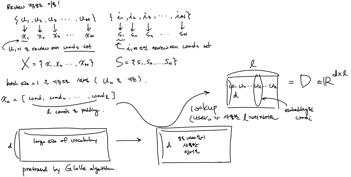
위의 수기 표현에서의 그림을 설명하면 다음과 같다.
user $u$ 가 사용한 word를 padding 하여 $l$ 개 의 word를 사용헀다고 하고, 모든 유저가 사용한 단어들에 대해 embedding 된 vector들(이 값들은 수많은 단어들에 대해 GloVe 알고리듬에 의해 pretrained 된 word embedding 값들은 초기값으로 하여 가져온다)에서 lookup 하여 $D \in \mathbb{R}^{d \times l} $를 가져오는 과정이다.
(여기서 $d$ 는 embedding dimension) \(D = [ \mathbf{w}_1, \mathbf{w}_2, ..., \mathbf{w}_l].\) 한국어 blog 설명
Local attention layer
local attention score 를 구할떄 sliding window $W_{L-a} \in \mathbb{R}^{ w \times d}$ 를 이용하여 convolution 연산을 함으로서 attention score들을 구하게 된다.
( window size $ w $ 과 word embedding vector $\mathbf{w}$ 는 다르다)
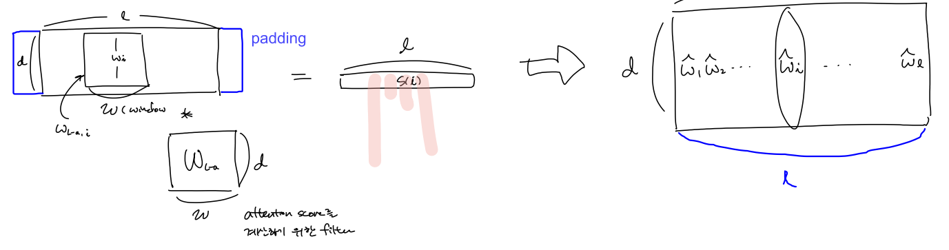
$delta(.)$ 는 $\mbox{sigmoid}$ 함수
$*$ 는 $ \mbox{convolution} $
\(\mathbf{w}_{L-a} \in \mathbb{R}^{w \times d} \\
\mathbf{W}_{L-a} \in \mathbb{R}^{w \times d} \\
b_{L-a} \in \mathbb{R} \\
\hat{D} \in \mathbb{R}^{d \times l}\)
따라서, 어떤 user $u$ 에 대해 local attention score가 반영된 word embedding matrix $\hat{D}$ 를 구할 수 있다.
Convolution operation
어떤 user $u$ 에 대해 $\hat{D}$ 가 주어지면 filter $ \mathbf{W}_c^j \in \mathbb{R}^{w \times d}$ ($j = 1, 2, …, f$)와의 convolution 연산을통해(pooling은 아직 하지 않는다) local attention이 word 에 대해 반영된 local contextual feature들을 계산할 수 있다.
특정 user가 사용한 $i$ 번쨰 단어에 대한 local contextual feature vector $\mathbf{c}_i \in \mathbb{R}^f$를 계산
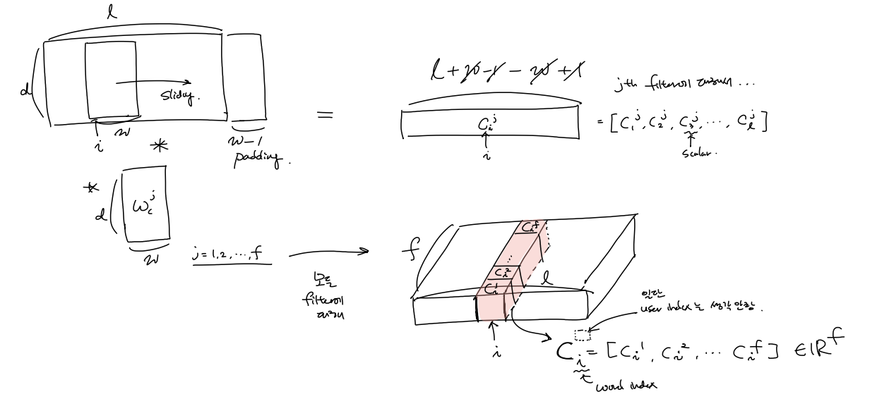
($c_i^j \in \mathbb{R}$, $\mathbf{c}_i \in \mathbb{R}^f$ ) \(\begin{aligned} c_i^j &= \mathbf{W}_c^j*\hat{D}(:,i:(i+w-1)) \color{green}~ {\mbox{//local contextual feature}} \\ \mathbf{c}_i &= [c_i^1, c_i^2, ...,c_i^f] \\ \end{aligned}\)
어떤 특정 user $u$에 대한 local contextual feature vector들과 item $i$에 대한 local contextual feature vector들은 다음과 같은 그림이 된다.
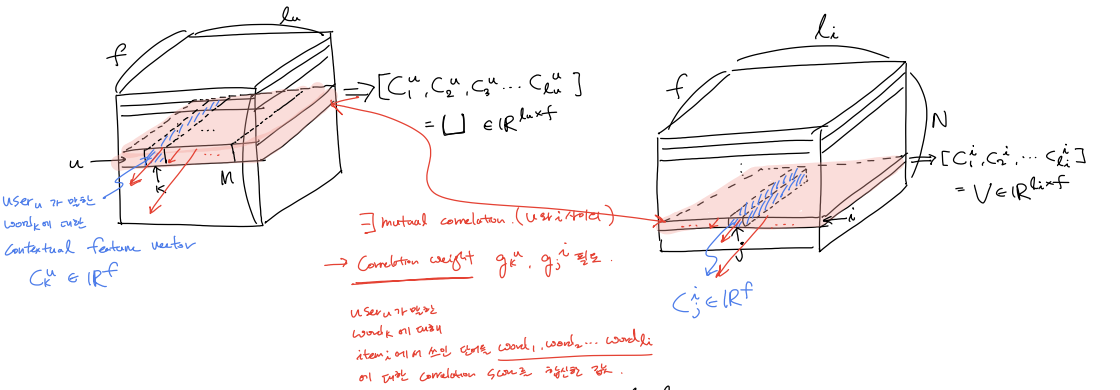
($\mathbf{c}_k^u \in \mathbb{R}^f$, $\mathbf{c}_j^i \in \mathbb{R}^f$, $k = 1,2,..,l_u$, $j = 1,2,..,l_i$, $u = 1,2,..,M$, $i = 1,2,..,N$)
\(\begin{aligned}
\mbox{for a (u,i) pair, } \\
\mathbf{U} &= [\mathbf{c}_1^u,\mathbf{c}_2^u, ..., \mathbf{c}_{l_u}^u ] \\
\mathbf{V} &= [\mathbf{c}_1^i,\mathbf{c}_2^i, ..., \mathbf{c}_{l_i}^i ]
\end{aligned}\)
이떄, $\mathbf{U}$ 와 $\mathbf{V}$ 사이의 mutual 한 관계가 있을 것이다.
Mutual attention layer
train record 는 $(u,i, r )$ 형태로 들어오는데 $u$ 가 쓴 review에서의 word들과 $i$에 쓰인 review에서의 words들의 feature사이의 correlation score 함수 $f_{relation-score}(\mathbf{c}_k^u, \mathbf{c}_j^i)$를 정의하여 user-itme mutual attention matrix $\mathbf{A}$를 계산 해두고, 이를 이용하여 correlation weight값 $g_k^u, g_j^i$들을 구해, 각 feature들에 이를 반영하고 싶은게 이 부분을 목적이다.
$f_{relation-score}(\mathbf{c}_k^u, \mathbf{c}_j^i) \in \mathbb{R} $ 는 $u$의 $word_k$ 와 $i$의 $word_j$ 사이의 correlation score를 의미한다. (왜냐하면 두 feature 사이의 유클리디안 distance 값의 역수이므로)
\(f_{relation-score}(\mathbf{c}_k^u, \mathbf{c}_j^i) = 1/(1+|\mathbf{c}_k^u - \mathbf{c}_k^u|)\)
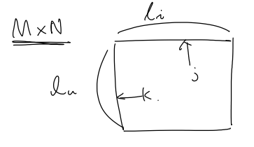
이때, $k \in [1, l_u]$, $j \in [1, l_i]$ 이므로 $\mathbf{A}[ 1 \le k \le l_u, 1 \le j \le l_i]$ 가 되고, $\mathbf{A}$ 의 종류는 $M \times N$ 개가 된다.
그렇게 계산해 놓은 $\mathbf{A}$ 를 이용하여 mutual correlation weight를 구한다.
$g_k^u $ 가 뜻하는 바는 $u$가 사용한 단어 $word_k$ 와 $i$에 사용된 단어 전부에 대한 correlation score를 aggregate한 값을 의미한다.
($g_k^u, g_j^i \in \mathbb{R}$) \(g_k^u = \sum{\mathbf{A}[k,:]} \\ g_j^i = \sum{\mathbf{A}[:,j]} \\\)
Local pooling layer
$g_k^u, g_j^i$ 를 이용하여 모든 local context feature 에 mutual correlation weight를 반영하여(feature 들간의 context도 반영하기 위해 padding과 함께 window단위로 convolution을 하여 구함) context feature with the weight of mutual attention $\mathbf{t}_k^u, \mathbf{t}_j^i $ 들을 구한다.
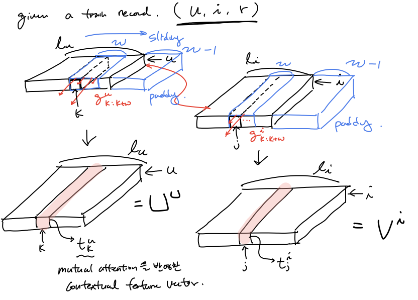
($t_k^u, t_j^i \in \mathbb{R}^f$)
\[t_k^u = \sum_{k=k:k+w}{g_k^u \mathbf{c}_k^u} \\ t_j^i = \sum_{k=k:k+w}{g_j^i \mathbf{c}_j^i} \\ \mathbf{U}^u = [t_1^u, t_2^u, ..., t_{l_u}^u] \\ \mathbf{V}^i = [t_1^i, t_2^i, ..., t_{l_i}^i] \\\]word들의 feature 간의 mutual correaltion를 생각한 context feature를 이용하여 user에 대한 feature 를 convolution과 mean pooling을 통해 구해보자
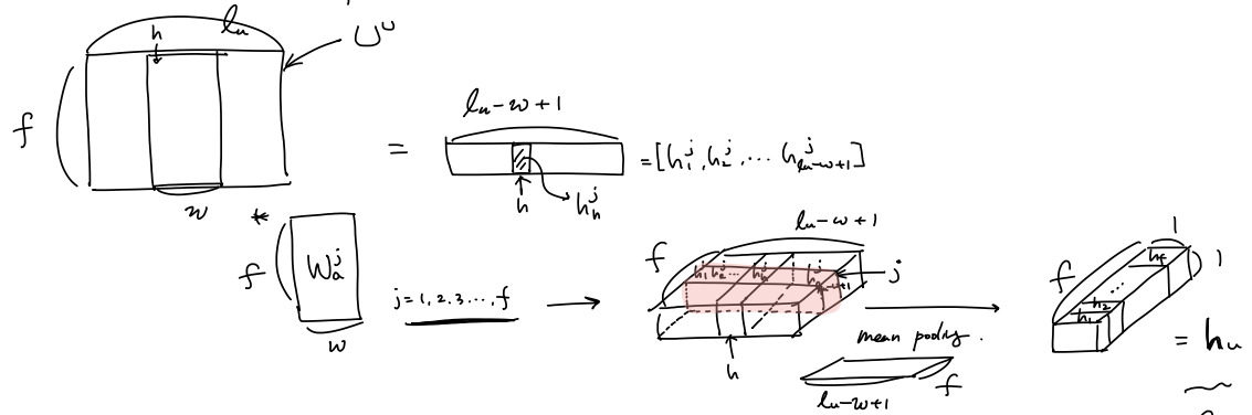
($ \mathbf{W}_a^j \in \mathbb{R}^{w \times f}, h_h^j \in \mathbb{R}, h_h \in \mathbb{R}, \mathbf{h}^u \in \mathbb{R}^f$)
\[h_h^j = \delta(\mathbf{W}_a^jU_{h:h+w-1}^u + b_a^j) \\ h_h = mean(h_1^j, h_2^j, ..., h_{l_u - w +1}^j) \\ \mathbf{h}^u = [h_1, ..., h_f]\]마지막으로 affine layer를 통과 시키자
($\mathbf{W}^u \in \mathbb{R}^{K \times f}, \mathbf{W}^u \in \mathbb{R}^{K \times f}$ ) \(\mathbf{h}^u = \delta(\mathbf{W}^u \mathbf{h}^u + b^u) \\ \mathbf{h}^i = \delta(\mathbf{W}^i \mathbf{h}^i + b^i)\) The final contextual feature with user-item correlation $\mathbf{h}^u, \mathbf{h}^i$ 를 얻을 수 있다.
Feature Interaction Module
user-item correlation 을 고려한 contextual feature $\mathbf{h}^u, \mathbf{h}^i$와 user와 item 각각에 대한 interaction features $\mathbf{p}_u, \mathbf{q}_i$ 를 얻는다. 이 heterogeneous 한 정보를 융합(fuse) 하여 포괄적인 user의 preference $\mathbf{u}^u$와 item에 대한 characteritics $ \mathbf{v}^i$를 얻는다. 그 다음 이 두 feature들을 concat 한 vector를 user-item feature $\mathbf{z}$라 한다.
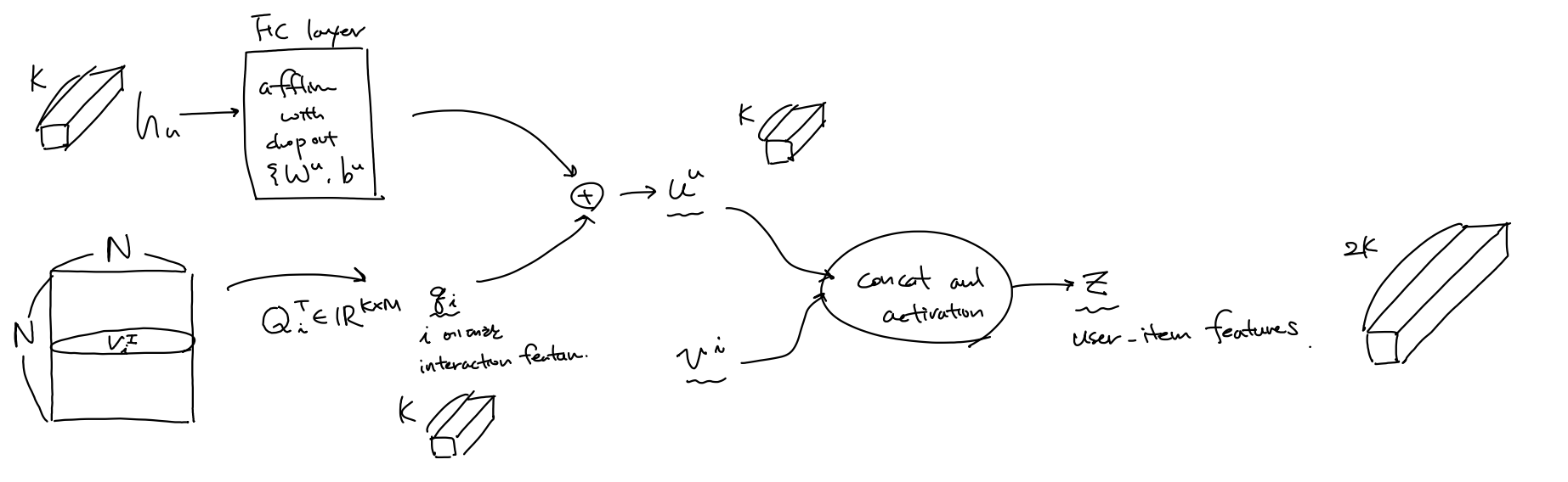
($ \mathbf{P}_u^T \in \mathbb{R}^{K \times M}, \mathbf{Q}_i^T \in \mathbb{R}^{K \times M}, [,] ~ \mbox{is concatenation}, \mathbf{u}^u \in \mathbb{R}^K, \mathbf{u}^u \in \mathbb{R}^K, \mathbb{z} \in \mathbb{R}^{2K}$ )
\[\mathbf{p}_u = \mathbf{P}_u^Tv_u^U \\ \mathbf{q}_i = \mathbf{Q}_i^Tv_i^I \\ \mathbf{u}^u = \mathbf{h}^u + \mathbf{q}_i \\ \mathbf{v}^i = \mathbf{h}^i + \mathbf{p}_u \\ \mathbf{z} = \delta[u,v]\]이제 high-order nonlinear interaction 를 capture 하는 방식을 통해 predicted rating을 구하는 데 있어서 서로 다른 두 feature 들간의 관계를 나타내는 $f(\mathbb{z})$ 를 기존 방식(DeepCoNN[WSDM’17])에서는 FM을 이용했지만 여기서는 MLP를 이용하여 Neural Net구조로 구한다.
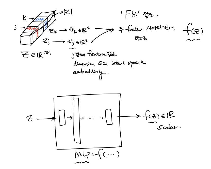
($\hat{r}_{u,i}, f(\mathbf{z}) \in \mathbb{R}$) \(\hat{r}_{u,i}(\mathbf{z}) = m_0 + \sum_{j=1}^{|\mathbf{z}|}{m_j}z_j + f(\mathbf{z}) \\ f(\mathbf{z}) = h^T\delta_L(W_L(...\delta_1(W_1f(\mathbf(z) + b_1)...)+b_L)\)
Training
loss function 은 regularization term을 추가하여 다음과 같다.
($\theta$ $\mbox{is all parameters}$) \(J = \sum_{(u,i) \in R} {(\hat{r}_{u,i} - r_{u,i})^2 + \lambda_{\theta} ||\theta||^2}\) Adam optimizer 를 이용하여 minibatch 단위로 training 한다.

Leave a comment