
Attention Mechanism
Attention Mechanism은 Neural Machine Translation, NMT 분야에서 Seq2seq(S2S)모델 의 성능을 높히기 위해 처음 사용되었다[1-2].
S2S model Notation
| name | representation | dimension | how to get |
|---|---|---|---|
| input | $x_{i=1,2.., T_x}$ | $x_i \in \mathbb{Z}_{+} $ | given |
| input’s hidden state | $h_{i=1, 2,..,T_x}$ | $h_i \in \mathbb{R} ^d$ | encoder’s output for each step |
| target | $y_{i=1, 2, .., T_y}$ | $y_i \in \mathbb{Z}_{+}$ | given |
| target’s hidden state | $s_{i=1, 2, .., T_y}$ | $s_i \in \mathbb{R} ^d$ | decoder’s output for each step |
| context vector | $c_{i=1, 2, .., T_x}$ | $c_i \in \mathbb{R} ^d$ | $\sum_{j=1}^{T_x}{\alpha_{ij}h_j}$ |
| alignment vector | $\alpha_{ij}$ $i\in [1, T_y]$ $j\in [1, T_x]$ |
$\alpha_{ij} \in \mathbb{R}$ | $\frac{exp(e_{ij})}{\sum_{k=1}^{T_x}e_{ik}}$ |
| energy | $e_{ij}$ $ i \in [1, T_y]$ $j\in [1, T_x]$ |
$e_{ij} \in \mathbb{R} $ | $align(s_{i-1}, h_j)$ |
- context vector $c_{i}$는 $y_i$에 대한 input’s hidden state에 대해 attention weights로 weight average된 벡터.
- attention weight $\alpha_{ij}$는 $e_{ij}$를 $j$축에 대해 softmax를 취한 값이며 $[0, 1]$의 확률값.
- energy $e_{ij}$는 decoder의 cell이 $s_i$를 output하고 $y_i$를 예측할 때 쓰는 $s_{i-1}$가 encoder의 $h_j$와 얼마나 유사한지 나타내는 scalar 값.
Description
w/o Attention
Attention Mechanism이 사용되지않은 Sequence to Sequence model은 다음과 같이 계산된다.
encoder에서 다음 그림과 같이 context vector를 decoder에게 넘겨줄때, 첫 time step에서만 넘겨주게 된다.
| overview | pytorch implementation |
|---|---|
 |
 |
1
2
3
4
5
6
7
8
9
10
11
12
13
14
15
16
17
18
19
20
class DecoderRNN(nn.Module):
    """ w/o attention mechanism. """
    def __init__(self, hidden_size, output_size):
        super(DecoderRNN, self).__init__()
        self.hidden_size = hidden_size

        self.embedding = nn.Embedding(output_size, hidden_size)
        self.gru = nn.GRU(hidden_size, hidden_size)
        self.out = nn.Linear(hidden_size, output_size)
        self.softmax = nn.LogSoftmax(dim=1)

    def forward(self, input, hidden):
        output = self.embedding(input).view(1, 1, -1)
        output = F.relu(output)
        output, hidden = self.gru(output, hidden)
        output = self.softmax(self.out(output[0]))
        return output, hidden

    def initHidden(self):
        return torch.zeros(1, 1, self.hidden_size, device=device)
with Attentnion
만약 decoder에서 output할 문장이 긴 문장이면 context vector의 영향이 적어 성능이 떨어질 수 있다.
이런 약점을 보완하고자, decoder에서 매 time step마다 다른 context vecter를 만들어 단어를 output하도록 하였다.
attention mechanism이 쓰이지 않은 기존 모델과 다른 점은
decoder에서 contect vector를 모두 같은 것을 쓰거나 단순히 전파되는 것이 아니라
매 time step마다 다른 context vecter를 만든다는 점이다.
다음 그림과 같이 각기 다른 context vector는 encoder의 전체 hidden state들과 decoder의 이전 hidden state 를 바탕으로 만든다.
(그림과 구현은 [1]의 방식을 기준으로 작성 되었으며, [14]에 각 논문들 별로 구체적인 구현과정을 visualization과 함께 설명하였다.)
| overview | animation | pytorch implementation |
|---|---|---|
 |
 |
 |
1
2
3
4
5
6
7
8
9
10
11
12
13
14
15
16
17
18
19
20
21
22
23
24
25
26
27
28
29
30
31
32
33
34
35
class AttnDecoderRNN(nn.Module):
    def __init__(self, hidden_size, output_size, dropout_p=0.1, max_length=MAX_LENGTH):
        super(AttnDecoderRNN, self).__init__()
        self.hidden_size = hidden_size
        self.output_size = output_size
        self.dropout_p = dropout_p
        self.max_length = max_length

        self.embedding = nn.Embedding(self.output_size, self.hidden_size)
        self.attn = nn.Linear(self.hidden_size * 2, self.max_length)
        self.attn_combine = nn.Linear(self.hidden_size * 2, self.hidden_size)
        self.dropout = nn.Dropout(self.dropout_p)
        self.gru = nn.GRU(self.hidden_size, self.hidden_size)
        self.out = nn.Linear(self.hidden_size, self.output_size)

    def forward(self, input, hidden, encoder_outputs):
        embedded = self.embedding(input).view(1, 1, -1)
        embedded = self.dropout(embedded)

        attn_weights = F.softmax(
            self.attn(torch.cat((embedded[0], hidden[0]), 1)), dim=1)
        attn_applied = torch.bmm(attn_weights.unsqueeze(0),
                                 encoder_outputs.unsqueeze(0))

        output = torch.cat((embedded[0], attn_applied[0]), 1)
        output = self.attn_combine(output).unsqueeze(0)

        output = F.relu(output)
        output, hidden = self.gru(output, hidden)

        output = F.log_softmax(self.out(output[0]), dim=1)
        return output, hidden, attn_weights

    def initHidden(self):
        return torch.zeros(1, 1, self.hidden_size, device=device)
Family of Attention Mechanism
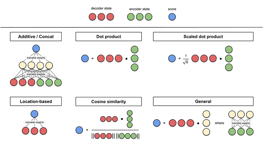
$e_{ij} = align(s_{i-1}, h_j)$를 계산하는 alignment model은 여러 Family 가 있다.
notation을 간결화 하기위해 $i-1$을 $t$로 치환하여 정리
| Name | alignment score function: $align(\mathbf{s}_t, \mathbf{h}_j)$ | citation |
|---|---|---|
| additive | $\mathbf{v}_a^\top tanh(\mathbf{W}_a[\mathbf{s}_t; \mathbf{h}_i])$ | Bahdanau2015 |
| Location-Base | $\alpha_{t,i} = softmax(\mathbf{W}_a \mathbf{s}_t) $ Note : This simplifies the softmax alignment max to only depend on the target position. |
Luong2015 |
| General | $\mathbf{s}_t^\top \mathbf{W}_a \mathbf{h}_i$ where $\mathbf{W}_a$ is a trainable weight matrix in the attention layer. |
Luong2015 |
| Dot-Product | $ \mathbf{s}_t^\top \mathbf{h}_i$ | Luong2015 |
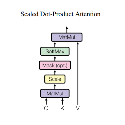
| Scaled Dot-Product | ${\mathbf{s}_t^\top \mathbf{h}_i}\over{\sqrt{n}}$ Note: very similar to dot-product attention except for a scaling factor; where n is the dimension of the source hidden state. |
Vaswani2017 |
어텐션 방식을 더 넓은 범위에서 다음과 같이 카테고리화 할 수 있다(서로 영역이 겹칠 수 있음).
| Name | How | citation |
|---|---|---|
| Self(or intra) | Relating different positions of the same input sequence. $x_{(:)} = y_{(:)}$ | Cheng2016 Vaswani2017 |
| Cross | works on different sequences; $x_{(:)} \neq y_{(:)}$ | |
| Global/Soft | Attending to the entire input state space. | Xu2015 |
| Local/hard | Attending to the part of input state space; $i.e.$ a patch of the input image. | Xu2015;Luong2015 |
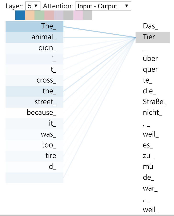
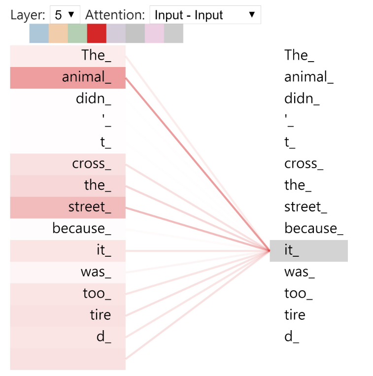
Cross vs Self
[4]를 바탕으로 설명하면 이해가 쉽다.
| cross | self(or intra) |
|---|---|
| works on different sequence | relate different positions of single sequence to compute its representation |
 |
 |
Soft vs Hard
[3]에서 기본적 아이디어 제안 됨. [3]은 image captioning을 목표로 하며 attention 구조 및 모델 overview는 다음과 같다.

[3]은 번역 문제가 아니라서 notation이 약간 다르다. 헷갈릴 수 있으니 정리하겠다.
| name | notation |
|---|---|
| a sub-section of an image | $y_{i=1, 2, …, n}$ after CNN |
| context | $C(= h_{t-1} )$ |
| summary | $Z$ |
어텐션 모델은 $y_{i=1, 2,…, n}$의 weighted arithmetic mean을 반환하며, weight는 주어진 context C에 대한 각 $y_i$의 연관도에 따라 설정된다.
| soft: deterministic | hard: stochastic |
|---|---|
| 모든 alignment vector를 반영하여 weight average | alignment vector값으로 확률적으로 샘플링 |
 |
 |
| * | soft | hard |
|---|---|---|
| 장점(+) | 모델이 스무스하고 미분가능(differentiable)함 | 인퍼런스에서 더 적은 계산 비용 |
| 단점(-) | 이미지가 클 때 계산비용이 큼 | 샘플링했기때문에 미분 불가능(non-differentiable) |
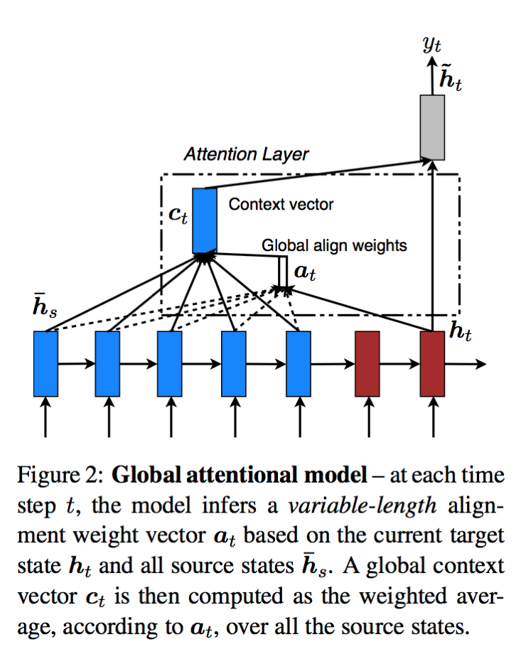
Global vs Local
[2]에서 아이디어가 처음 제안 됨.
| global | local |
|---|---|
 |
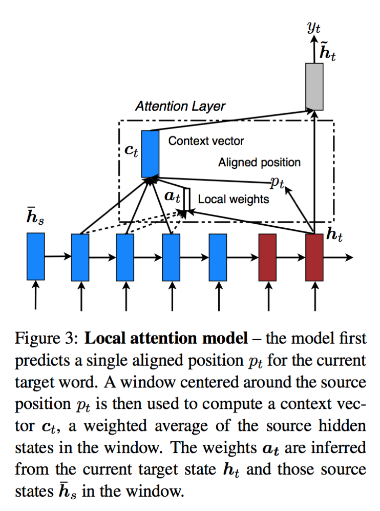 |
| to generate a target word, consider all source words basically soft attention |
to generate a target word, first predicts a source word position use a window around this position to compute the target word blend of soft and hard (to make hard attention differentiable) |
| 근본적으로 global | alignment vector들을 구할 기준이 되는 position을 샘플링하는게 아니라 예측함으로써 미분가능해지며, 에측한 위치에서 window 크기 내에 들어오는 source word 들을 고려하여 alignment vectors를 만들고 aggregate해서 context vector를 만든다. |
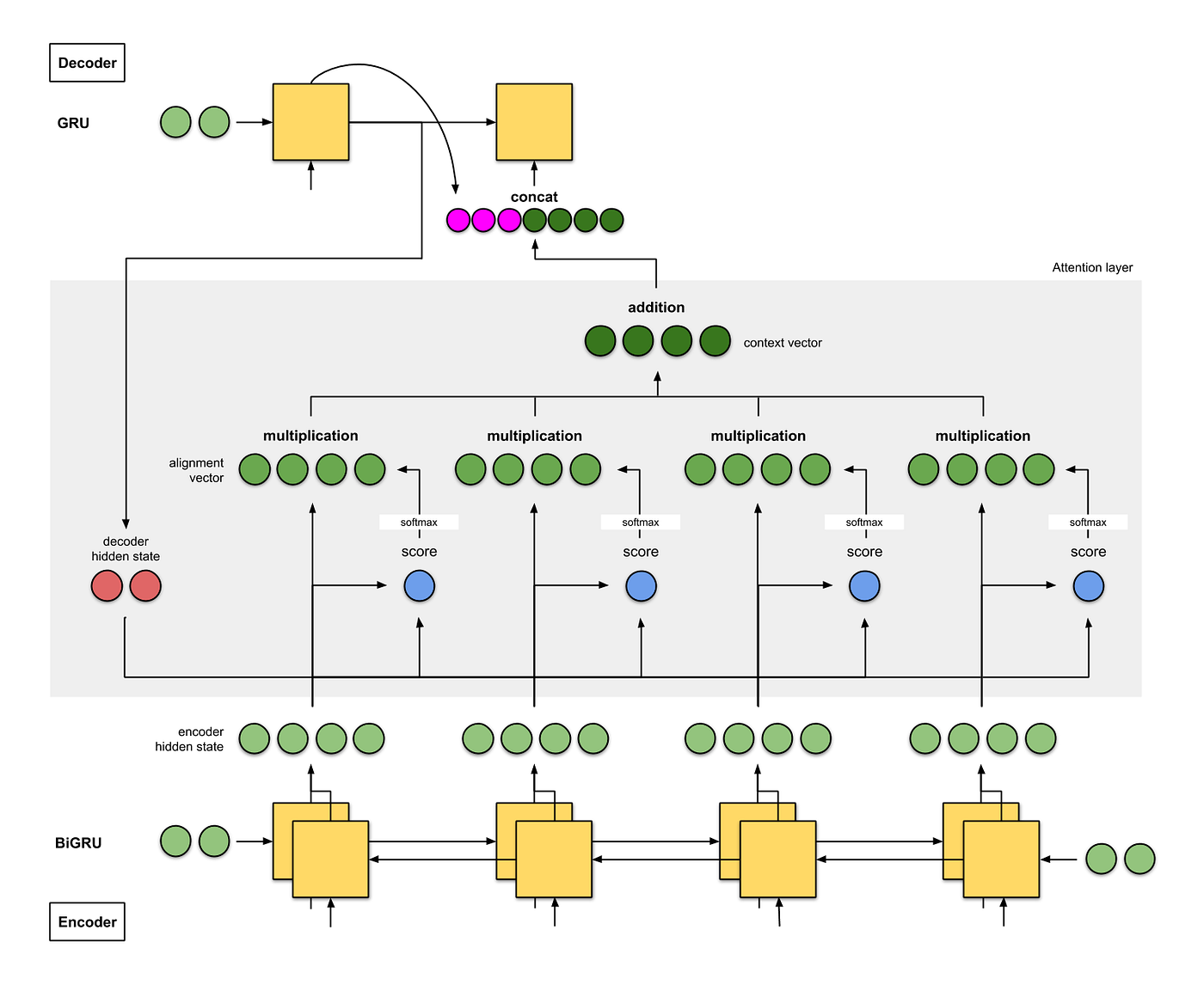
soft와 global 의 구현 차이
| soft | global |
|---|---|
 |
 |
| Bahdanau, ICLR’15 | Luong, EMNLP’15 |
| decoder GRU, encoder는 BiGRU 사용 | LSTM 사용 |
| alignment model: Scaled Dot-Product | Scaled Dot-Product, General, Dot-Product 실험 |
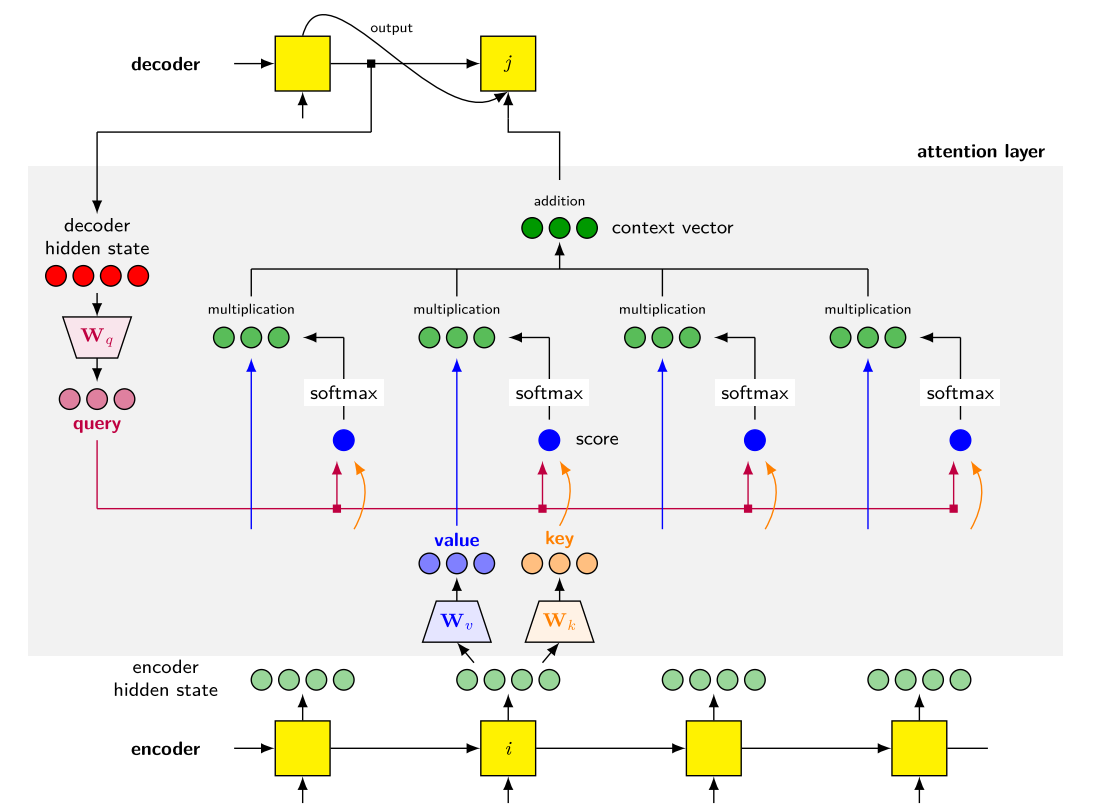
Key-Value
다음 그림과 같이 key, query, value 로 설명가능하다.
간략히 설명 하면 다음과 같다.
| name | description | dimension |
|---|---|---|
| query | (projected) decoder hidden state | $\mathbb{R}^{T_y \times d_q}$ |
| key | (projected) encoder hidden state (for attn weight computation); attention information | $\mathbb{R}^{T_x \times d_k}$ |
| value | (projected) encoder hidden state (for context vector buildup); content information | $\mathbb{R}^{T_x \times d_v}$ |
| context vector(outcome) | weight sum of values, where each weight is output of function(query, key) | $\mathbb{R}^{T_y \times d_v}$ |
다음 그림처럼 query, key를 바탕으로 alignment vector 를 구하고(scaled dot product방식) value에 적용하므로써 context vector를 구한다. 그림과 같이 계산하려면 제약사항은 $d_k = d_q$ 이어야 hadamard product가 가능하다.
Multi-Head
[4] 에서 다음 그림과 같은 Transformer 구조를 사용하였고, 성능을 비약적으로 높혔다.
- 위와 같은 Key-Value Attention Mechanism을 효율적(병렬적)으로 하였다.
- Multi-Head를 사용하였다.
![]()
| LSTM | Transformer |
|---|---|
| decoder에서 previous step에 대한 hidden state를 구해야 current step의 계산을 할 수있다 | 한번에 decoder의 모든 step을 계산할 수 있다 |
| 병렬 계산 불가능 | 병렬 계산 가능 |
이 곳에서 tensorflow를 사용하여 코드 단계에서 NMT 를 학습하고 예측하는 tutorial 를 line by line으로 실행해 보았다.
Reference
Papers
[1] Neural Machine Translation by Jointly Learning to Align and Translate arXiv Bahdanau, ICLR’15
[2] Effective Approaches to Attention-based Neural Machine Translation arXiv Luong, EMNLP’15
[3] Show, Attend and Tell: Neural Image Caption Generation with Visual Attention arXiv Xu, ICML’15
[4] Attention Is All You Need arXiv Vaswani, NIPS’17
Documents
[11] NLP 흐름 정리
[12] S2S 모델에 대한 visualization 이 잘되어있는 blog
[13] Pytorch S2S Tutorial, 가장 구체적이게 묘사한다, 구현 시 이 방식으로 할 것
[14] Attention 방법론에 대한 정리가 가장 잘 되어있다, medium english, DL 수업 참고자료; tistory, korean
[15] Attention 방법론에 대한 정리 v2, english; yjucho’s blog, korean)
[16] Soft vs Hard attention 정리 blog, english; blog, korean
[17] [2]논문을 정리, Global vs Local 비교 설명 포함, korean

Leave a comment