
1
2
3
4
5
6
7
import numpy as np
import pandas as pd
import random
from sklearn.metrics import confusion_matrix
from sklearn.metrics import precision_score
from sklearn.metrics import recall_score
import matplotlib.pyplot as plt
Unsupervised Clustering
Among Clustering methods, K-means and K-medoiod belong to Unsupervised Learning.
Also, they are in EM algorithm categories.
Notations
$K$ = # of clusters
$N$ = # of dataset
$t$ = # of iteration
$p$ = the dimension of the data
$m_k$ = # a centroid of cluster $k$
The objective of $K$-means clustering and $K$-medoids is same, which is to find $K$ clustering given dataset by minimizing the cost as you can see below.
\(\underset{C}{\operatorname{argmin}}\sum_{k=1}^{K}{\sum_{x \in C_k}{d(x,m_k)}}\) where $d(x,m_k)$ means squared Euclidean distance
The big difference of K-means and K-mediods is the way how the $m_k$ are updated
Load Toy example, and Test dataset
1
2
3
4
5
6
7
8
9
10
11
12
13
# Load data
toy = np.load('./data/clustering/data_4_1.npy') # data_1, for visualization
test = np.load('./data/clustering/data_4_2.npz') # data_2, for test
X = test['X']
y = test['y']

# Sanity check
print('data shape: ', toy.shape) # (1500, 2)
print('X shape: ', X.shape) # (1500, 6)
print('y shape: ', y.shape) # (1500,)

df_toy = pd.DataFrame(toy, columns=['f1', 'f2'])
df_toy  # toy example does not have ground truth label.
1
2
3
4
data shape:  (1500, 2)
X shape:  (1500, 6)
y shape:  (1500,)
| f1 | f2 | |
|---|---|---|
| 0 | 12.630551 | 2.254497 |
| 1 | 2.452222 | -7.716821 |
| 2 | 3.408706 | -5.010174 |
| 3 | 7.444588 | -0.194091 |
| 4 | 0.929980 | -7.329755 |
| ... | ... | ... |
| 1495 | 3.054506 | -3.679957 |
| 1496 | 0.282762 | -8.043163 |
| 1497 | 3.323046 | -6.140348 |
| 1498 | 0.779888 | -8.446471 |
| 1499 | 1.227547 | -9.741289 |
1500 rows × 2 columns
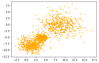
Visualize toy examples
1
2
toy = df_toy.to_numpy()
plt.scatter(toy[:,0], toy[:,-1], color = 'orange', s = 7)
1
<matplotlib.collections.PathCollection at 0x7fa4de1f9410>
1
2
3
4
5
features = ['f1', 'f2', 'f3', 'f4', 'f5', 'f6']
test = pd.DataFrame(X, columns=features)
test = pd.merge(left=test, right=pd.DataFrame(y, columns=['label']), on=test.index)
test = test[features + ['label']]
test
| f1 | f2 | f3 | f4 | f5 | f6 | label | |
|---|---|---|---|---|---|---|---|
| 0 | 4.200999 | -0.506804 | -0.024489 | -0.039783 | 0.067635 | -0.029724 | 2 |
| 1 | 4.572715 | 1.414097 | 0.097670 | 0.155350 | -0.058382 | 0.113278 | 0 |
| 2 | 9.183954 | -0.163354 | 0.045867 | -0.257671 | -0.015087 | -0.047957 | 1 |
| 3 | 8.540300 | 0.308409 | 0.007325 | -0.068467 | -0.130611 | -0.016363 | 2 |
| 4 | 8.995599 | 1.275279 | -0.015923 | 0.062932 | -0.072392 | 0.034399 | 0 |
| ... | ... | ... | ... | ... | ... | ... | ... |
| 1495 | 3.054506 | -3.679957 | 0.042136 | 0.012698 | 0.121173 | 0.076322 | 1 |
| 1496 | 0.282762 | -8.043163 | 0.049892 | -0.055319 | -0.031131 | 0.213752 | 0 |
| 1497 | 3.323046 | -6.140348 | -0.104975 | -0.257898 | -0.000928 | -0.094528 | 1 |
| 1498 | 0.779888 | -8.446471 | 0.105319 | 0.166633 | 0.018645 | 0.108826 | 0 |
| 1499 | 1.227547 | -9.741289 | 0.010518 | -0.121976 | -0.020301 | -0.077125 | 0 |
1500 rows × 7 columns
1
2
3
# exploration
print("min info:\n", test.min())
print("max info:\n", test.max())
1
2
3
4
5
6
7
8
9
10
11
12
13
14
15
16
17
18
19
min info:
 f1       -2.802532
f2      -11.719322
f3       -0.291218
f4       -0.378744
f5       -0.336366
f6       -0.383337
label     0.000000
dtype: float64
max info:
 f1       17.022084
f2        7.953588
f3        0.402071
f4        0.310862
f5        0.316762
f6        0.342837
label     2.000000
dtype: float64
$K$-means Clustering
Procedure
- Initialization: Choose $K$ initial cluster centriods
- Expectation
- Compute point-to-cluster-centroid distances of all data points to each centroid
- Assign each point to the cluster with the closest centroid.
\(\text{assign } x_i \text{ to the cluster label } C_k \text{such that } k = \underset{k}{\operatorname{argmin}}{d(x_i, m_k)} ,~ \forall i \in [1, 2, ..., N]\)
- Maximization
- Update the centroid values: the average of the points in each cluster
- Repeat 2, 3 until satisfying stopping condition: converge(by computing loss) or iteration over.
so, the time complexity is $O(tpKN)$
Going through iteration, loss is monotonically decreases, and finally loss is converged.
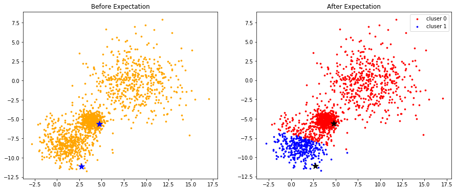
Initialization
Initialize $K$ centriods and visualize it to 2D space for given toy examples.
star stickers means $K$ centriods.
1
2
3
4
5
6
7
8
9
10
K = 2
data = toy
p = np.size(data, axis=1)  # the number of features.
print("the number of features:", p)
centroids = data[random.sample(range(len(data)), K), :]  # [K, p], choose K centroids.
print(centroids)
# 2D visualization
plt.scatter(data[:, 0], data[:, 1], c='orange', s=7)
plt.scatter(centroids[:,0], centroids[:,1], marker='*', c='b', s=150)
plt.show()
1
2
3
4
the number of features: 2
[[  4.77497947  -5.60411467]
 [  2.744412   -11.12111773]]

Expectation
1
2
3
4
5
6
7
8
9
10
11
12
13
14
15
16
17
18
19
20
21
22
23
def distance_matrix(data, centroids, verbose=False):
    """ using broadcasting of numpy, compute distance matrix for each cluster.
    Args:
        data: [N, p]
        centroids: [K, p]
    notations:
        :N: the number of examples,
        :K: the number of clusters,
        :p: the feature dimension of each sample.
    return distance matrix, of shape=[N, K]"""
    squares = ((data[:, :, np.newaxis] - centroids.T[np.newaxis, :]) ** 2)  # [N, p, K]
    distances = np.sum(squares, axis=1)  # [N, K]
    if verbose:
        # visualize distance matrix for each cluster.
        df = pd.DataFrame(distances, columns=['C1', 'C2'])
        print(df)
    return distances

def expectation(data, centroids):
    """ Assigning each value to its closest cluster label. """
    distances = distance_matrix(data, centroids)  # [N, K]
    clusters = np.argmin(distances, axis=1) # [N,]
    return clusters
1
distance_matrix(data, centroids, verbose=True)
1
2
3
4
5
6
7
8
9
10
11
12
13
14
15
              C1          C2
0     123.467777  276.642807
1       9.858734   11.674608
2       2.219469   37.784922
3      36.395165  141.491565
4      17.761854   17.666598
...          ...         ...
1495    6.662411   55.467025
1496   26.128970   15.533526
1497    2.395656   25.142883
1498   24.039747   11.013091
1499   29.700489    4.204808

[1500 rows x 2 columns]
1
2
3
4
5
6
7
array([[123.46777735, 276.64280678],
       [  9.85873415,  11.67460837],
       [  2.21946911,  37.7849224 ],
       ...,
       [  2.39565643,  25.14288287],
       [ 24.03974697,  11.01309085],
       [ 29.70048881,   4.20480814]])
1
2
clusters = expectation(data, centroids)
clusters  # [N,]
1
array([0, 0, 0, ..., 0, 1, 1])
Visualize the result of expectation step
1
2
3
4
5
6
7
8
9
10
11
12
13
14
colors = ['r', 'b', 'g', 'y', 'c', 'm']
fig, (ax1, ax2) = plt.subplots(nrows=1, ncols=2, figsize=(15, 6))

ax1.scatter(data[:, 0], data[:, 1], c='orange', s=7)
ax1.scatter(centroids[:,0], centroids[:,1], marker='*', c='b', s=150)
ax1.set_title("Before Expectation")

for k in range(K):
    group = np.array([data[j] for j in range(len(data)) if clusters[j] == k])  # [*, p]
    ax2.scatter(group[:, 0], group[:, 1], s=7, c=colors[k], label='cluser {}'.format(k))
    ax2.legend()
ax2.scatter(centroids[:,0], centroids[:,1], marker='*', c='#050505', s=150)
ax2.set_title("After Expectation")
plt.show()
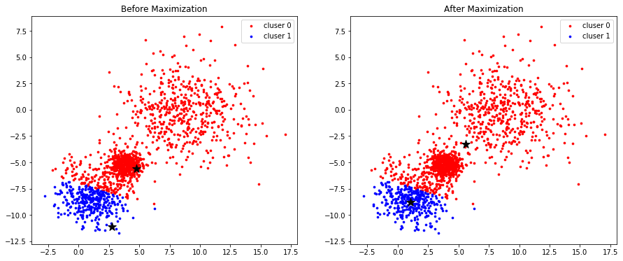
Maximization
1
2
3
4
5
6
7
def maximization(data, clusters, K):
    """ update centroids by taking the average value of each group. """
    centroids = np.zeros((K, np.size(data, axis = 1)))
    for k in range(K):
        group = np.array([data[j] for j in range(len(data)) if clusters[j] == k])  # [*, p]
        centroids[k] = np.mean(group, axis=0)
    return centroids
1
2
new_centroids = maximization(data, clusters, K)
new_centroids  # [K, p]
1
2
array([[ 5.59722207, -3.28657162],
       [ 1.03157988, -8.83044793]])
1
2
3
4
5
6
7
8
9
10
11
12
13
14
15
16
17
fig, (ax1, ax2) = plt.subplots(nrows=1, ncols=2, figsize=(15, 6))

for k in range(K):
    group = np.array([data[j] for j in range(len(data)) if clusters[j] == k])  # [*, p]
    ax1.scatter(group[:, 0], group[:, 1], s=7, c=colors[k], label='cluser {}'.format(k))
    ax1.legend()
ax1.scatter(centroids[:, 0], centroids[:, 1], marker='*', c='#050505', s=150)
ax1.set_title("Before Maximization")

for k in range(K):
    group = np.array([data[j] for j in range(len(data)) if clusters[j] == k])  # [*, p]
    ax2.scatter(group[:, 0], group[:, 1], s=7, c=colors[k], label='cluser {}'.format(k))
    ax2.legend()
ax2.scatter(new_centroids[:, 0], new_centroids[:,1 ], marker='*', c='#050505', s=150)
ax2.set_title("After Maximization")

plt.show()
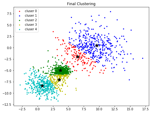
Compute Loss and repeat until converge
1
data.shape
1
(1500, 2)
1
2
3
4
5
6
7
8
def cost(data, clusters, centroids):
    K = len(centroids)
    loss = 0
    for k in range(K):
        group = np.array([data[j] for j in range(len(data)) if clusters[j] == k])  # [*, p]
        squares = (group - centroids[k][np.newaxis, :]) ** 2  # [*(# of sample in group[k]), p]
        loss += np.sum(np.sum(squares, axis=1), axis=0) # scalar
    return loss
1
2
3
4
5
6
7
8
9
10
11
12
13
14
15
16
17
18
def kmeans(data, K, iteration=10, bound=1e-7, verbose=False):
    # Initialization
    centroids = data[random.sample(range(len(data)), K), :]  # [K, p], choose K centroids.
    # Repeat EM algorithm
    error = 1e7
    while iteration:
        clusters = expectation(data, centroids)  # [N,]
        centroids = maximization(data, clusters, K)  # [K, p]
        loss = cost(data, clusters, centroids) # scalar
        if verbose: print("loss: {}".format(loss))
        if (error - loss) < bound:
            if verbose: print(error - loss)
            if verbose: print("converge")
            break
        error = loss
        iteration -= 1

    return clusters, centroids
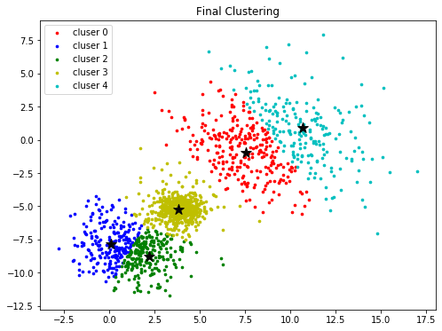
1
2
K = 5
clusters, centroids = kmeans(data, K, verbose=True)
1
2
3
4
5
6
7
8
9
10
11
loss: 7990.191121047926
loss: 7212.691330989318
loss: 7152.881427488944
loss: 7130.270405265313
loss: 7116.576976812909
loss: 7096.425347518904
loss: 7055.719485522531
loss: 6954.189159846061
loss: 6722.085830042569
loss: 6330.968027295821
1
2
3
4
5
6
7
8
9
colors = ['r', 'b', 'g', 'y', 'c', 'm']
fig, ax = plt.subplots(nrows=1, ncols=1, figsize=(8, 6))
for k in range(K):
    group = np.array([data[j] for j in range(len(data)) if clusters[j] == k])  # [*, p]
    ax.scatter(group[:, 0], group[:, 1], s=7, c=colors[k], label='cluser {}'.format(k))
    ax.legend()
ax.scatter(centroids[:, 0], centroids[:,1 ], marker='*', c='#050505', s=150)
ax.set_title("Final Clustering")
plt.show()
$K$-medoids Clustering
Procedure
- Initialization: same with $K$-means
- Expectation
- same with $K$-means \(\text{assign } x_i \text{ to the cluster label } C_k \text{such that } k = \underset{k}{\operatorname{argmin}}{d(x_i, m_k)} ,~ \forall i \in [1, 2, ..., N]\)
- Maximization
- For a given cluster assignment $C$, find a data point in each group that minimizes the sum of distances to other, and update the point as a centroid in the group.
points in that group
$C(i)=k$ means the index $i$ of $x_i \in C_k$ \(m_k = x_{i_k^*}\) \(i_k^* = \underset{i:C(i)=k}{\operatorname{argmin}}{\sum_{C(j)=k}{d(x_i, x_j)}}\)
- For a given cluster assignment $C$, find a data point in each group that minimizes the sum of distances to other, and update the point as a centroid in the group.
points in that group
- Repeat 2, 3 until satisfying stopping condition: same with $K$-means
so, the time complexity is $O(tdN^2)$
Implement maximization of $K$-medoids
1
2
3
4
5
6
7
8
9
10
11
12
13
14
15
def maximization_v2(data, clusters, K):
    """ update centroids by taking the average value of each group.
    Description: a**2 - 2ab + b**2 technique used for computing pairwise distance. """
    centroids = np.zeros((K, np.size(data, axis = 1)))
    for k in range(K):
        group = np.array([data[j] for j in range(len(data)) if clusters[j] == k])  # [G, p]
        asquares = np.sum(np.square(group), axis=1)  # [G,]
        bsquares = np.sum(np.square(group), axis=1)  # [G,]
        ab = np.einsum('ip,jp->ij', group, group)  # [G, G]
        # pairwise distances in the group k
        distances = asquares[:, np.newaxis] - 2 * ab + bsquares[np.newaxis, :] # [G, G]
        sum_dist = np.sum(distances, axis=1)
        i = np.argmin(sum_dist, axis=0)  # this is i_k^*
        centroids[k] = group[i]  # update centroid
    return centroids
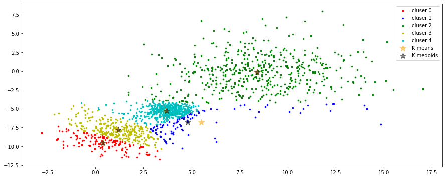
Visualization of different computation between K-means and K-mediods.
1
2
3
4
5
6
7
8
9
10
11
12
13
14
15
16
17
18
19
20
21
22
23
24
25
fig, ax = plt.subplots(nrows=1, ncols=1, figsize=(15, 6))

# initialization
centroids = data[random.sample(range(len(data)), K), :]  # [K, p], choose K centroids.

# expectation
clusters = expectation(data, centroids)

# maximization of K-means
centroids_v1 = maximization(data, clusters, K)

# maximization of K-medoids
centroids_v2 = maximization_v2(data, clusters, K)

for k in range(K):
    group = np.array([data[j] for j in range(len(data)) if clusters[j] == k])  # [*, p]
    ax.scatter(group[:, 0], group[:, 1], s=7, c=colors[k], label='cluser {}'.format(k))
    ax.legend()
ax.scatter(centroids_v1[:,0], centroids_v1[:,1], c='orange', marker='*', s=150,
            label='K means', alpha=0.5)
ax.legend()
ax.scatter(centroids_v2[:,0], centroids_v1[:,1], c='black', marker='*', s=150,
            label='K medoids', alpha=0.5)
ax.legend()
plt.show()
Implement overall algorithm
1
2
3
4
5
6
7
8
9
10
11
12
13
14
15
16
17
18
def kmedoids(data, K, iteration=10, bound=1e-7, verbose=False):
    # Initialization
    centroids = data[random.sample(range(len(data)), K), :]  # [K, p], choose K centroids.
    # Repeat EM algorithm
    error = 1e7
    while iteration:
        clusters = expectation(data, centroids)  # [N,]
        centroids = maximization_v2(data, clusters, K)  # [K, p]
        loss = cost(data, clusters, centroids) # scalar
        if verbose: print("loss: {}".format(loss))
        if (error - loss) < bound:
            if verbose: print(error - loss)
            if verbose: print("converge")
            break
        error = loss
        iteration -= 1

    return clusters, centroids
1
2
K = 5
clusters, centroids = kmedoids(data, K, verbose=True)
1
2
3
4
5
6
7
8
9
10
11
loss: 6933.893463699935
loss: 5892.018779804686
loss: 5779.071902042521
loss: 5730.8803618351485
loss: 5668.112584773427
loss: 5630.283712467555
loss: 5614.363123046829
loss: 5610.936338275873
loss: 5610.685620916394
loss: 5609.612766647277
1
2
3
4
5
6
7
8
9
colors = ['r', 'b', 'g', 'y', 'c', 'm']
fig, ax = plt.subplots(nrows=1, ncols=1, figsize=(8, 6))
for k in range(K):
    group = np.array([data[j] for j in range(len(data)) if clusters[j] == k])  # [*, p]
    ax.scatter(group[:, 0], group[:, 1], s=7, c=colors[k], label='cluser {}'.format(k))
    ax.legend()
ax.scatter(centroids[:, 0], centroids[:,1 ], marker='*', c='#050505', s=150)
ax.set_title("Final Clustering")
plt.show()
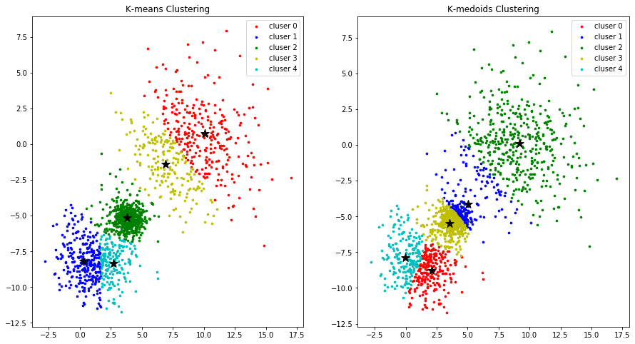
Compare Two methods
1
2
3
4
5
6
K = 5
%timeit kmeans(data, K, verbose=False)
%timeit kmedoids(data, K, verbose=False)

clusters_v1, centroids_v1 = kmeans(data, K, verbose=False)
clusters_v2, centroids_v2 = kmedoids(data, K, verbose=False)
1
2
3
58.2 ms ± 1.34 ms per loop (mean ± std. dev. of 7 runs, 10 loops each)
96.6 ms ± 7.68 ms per loop (mean ± std. dev. of 7 runs, 10 loops each)
1
2
3
4
5
6
7
8
9
10
11
12
13
14
15
16
colors = ['r', 'b', 'g', 'y', 'c', 'm']
fig, (ax1, ax2) = plt.subplots(nrows=1, ncols=2, figsize=(15, 8))
for k in range(K):
    group_v1 = np.array([data[j] for j in range(len(data)) if clusters_v1[j] == k])  # [*, p]
    ax1.scatter(group_v1[:, 0], group_v1[:, 1], s=7, c=colors[k], label='cluser {}'.format(k))
    ax1.legend()

    group_v2 = np.array([data[j] for j in range(len(data)) if clusters_v2[j] == k])  # [*, p]
    ax2.scatter(group_v2[:, 0], group_v2[:, 1], s=7, c=colors[k], label='cluser {}'.format(k))
    ax2.legend()

ax1.scatter(centroids_v1[:, 0], centroids_v1[:,1 ], marker='*', c='#050505', s=150)
ax2.scatter(centroids_v2[:, 0], centroids_v2[:,1 ], marker='*', c='#050505', s=150)
ax1.set_title("K-means Clustering")
ax2.set_title("K-medoids Clustering")
plt.show()
Test cases
1
test
| f1 | f2 | f3 | f4 | f5 | f6 | label | |
|---|---|---|---|---|---|---|---|
| 0 | 4.200999 | -0.506804 | -0.024489 | -0.039783 | 0.067635 | -0.029724 | 2 |
| 1 | 4.572715 | 1.414097 | 0.097670 | 0.155350 | -0.058382 | 0.113278 | 0 |
| 2 | 9.183954 | -0.163354 | 0.045867 | -0.257671 | -0.015087 | -0.047957 | 1 |
| 3 | 8.540300 | 0.308409 | 0.007325 | -0.068467 | -0.130611 | -0.016363 | 2 |
| 4 | 8.995599 | 1.275279 | -0.015923 | 0.062932 | -0.072392 | 0.034399 | 0 |
| ... | ... | ... | ... | ... | ... | ... | ... |
| 1495 | 3.054506 | -3.679957 | 0.042136 | 0.012698 | 0.121173 | 0.076322 | 1 |
| 1496 | 0.282762 | -8.043163 | 0.049892 | -0.055319 | -0.031131 | 0.213752 | 0 |
| 1497 | 3.323046 | -6.140348 | -0.104975 | -0.257898 | -0.000928 | -0.094528 | 1 |
| 1498 | 0.779888 | -8.446471 | 0.105319 | 0.166633 | 0.018645 | 0.108826 | 0 |
| 1499 | 1.227547 | -9.741289 | 0.010518 | -0.121976 | -0.020301 | -0.077125 | 0 |
1500 rows × 7 columns
1
2
3
4
5
data = test.to_numpy()
y = data[:, -1]
data = data[:, :-1]
K = 3
y.shape, data.shape
1
((1500,), (1500, 6))
1
2
clusters_v1, centroids_v1 = kmeans(data, K, iteration=100, verbose=False)
clusters_v2, centroids_v2 = kmedoids(data, K, iteration=100, verbose=False)
1
2
confusion1 = confusion_matrix(clusters_v1, y)
confusion2 = confusion_matrix(clusters_v2, y)
1
2
3
cluster_labels_true = ['c0', 'c1', 'c2']
cluster_labels_pred = ['g0', 'g1', 'g2']
pd.DataFrame(confusion1, index=cluster_labels_true, columns=cluster_labels_pred)
| g0 | g1 | g2 | |
|---|---|---|---|
| c0 | 9 | 13 | 456 |
| c1 | 59 | 487 | 44 |
| c2 | 432 | 0 | 0 |
1
pd.DataFrame(confusion2, index=cluster_labels_true, columns=cluster_labels_pred)
| g0 | g1 | g2 | |
|---|---|---|---|
| c0 | 9 | 13 | 453 |
| c1 | 48 | 487 | 47 |
| c2 | 443 | 0 | 0 |
The K-average ans K-method is an unsupervised method.
Therefore, the label order may not match the actual label.
So you need to adjust the order before assessing the performance.
1
2
3
4
5
6
7
def change(clusters, confusion):
    reorder = confusion.argmax(axis=-1)
    for i in range(len(clusters)):
        clusters[i] = reorder[clusters[i]]

change(clusters_v1, confusion1)
change(clusters_v2, confusion2)
1
2
3
confusion1 = confusion_matrix(clusters_v1, y)
confusion2 = confusion_matrix(clusters_v2, y)
pd.DataFrame(confusion1, index=cluster_labels_true, columns=cluster_labels_pred)
| g0 | g1 | g2 | |
|---|---|---|---|
| c0 | 432 | 0 | 0 |
| c1 | 59 | 487 | 44 |
| c2 | 9 | 13 | 456 |
1
pd.DataFrame(confusion2, index=cluster_labels_true, columns=cluster_labels_pred)
| g0 | g1 | g2 | |
|---|---|---|---|
| c0 | 443 | 0 | 0 |
| c1 | 48 | 487 | 47 |
| c2 | 9 | 13 | 453 |
1
2
3
4
5
6
7
precision_v1 = precision_score(y_true=y, y_pred=clusters_v1, average='macro')
precision_v2 = precision_score(y_true=y, y_pred=clusters_v2, average='macro')
print(precision_v1, precision_v2)

recall_v1 = recall_score(y_true=y, y_pred=clusters_v1, average='macro')
recall_v2 = recall_score(y_true=y, y_pred=clusters_v2, average='macro')
print(recall_v1, recall_v2)
1
2
3
0.9264662080703495 0.930151323325496
0.9166666666666666 0.922
1
2
3
4
f1_v1 = 2 * (precision_v1 * recall_v1) / (precision_v1 + recall_v1)
f1_v2 = 2 * (precision_v2 * recall_v2) / (precision_v2 + recall_v2)

print(f1_v1, f1_v2)
1
2
0.9215403863406526 0.9260577246639942
Summary
The objective of K-means clustering and K-medoids is same, which is to find K clustering given dataset by minimizing the cost as you can see below.
\(\underset{C}{\operatorname{argmin}}\sum_{k=1}^{K}{\sum_{x \in C_k}{d(x,m_k)}}\)
In this situation, the big difference of K-means and K-mediods is the way how the $m_k$ are updated
- $K$-means algorithm
some properties:- sensitive to initial seed points
- susceptible to outlier, density, distribution
- not possible for computing clusters with non-convex shapes
- $K$-mediod algorithm
some properties:- applies well when dealing with categorical data, non-vector space data
- applies well when data point coordinates are not available, but only pair-wise distances are available

Leave a comment