
1
2
3
4
5
import torch
import seaborn as sns
import numpy as np
import matplotlib.pyplot as plt
import pdb
beta 분포와 normal 분포의 차이
우리는 보통 두 분포의 유사도를 비교하며 파라미터를 찾을 때 KL divergence를 사용한다.
하지만 kl divergence두 분포의 parameter 를 정확히 알 때만 계산이 가능하다.
그래서 관측값으로 부터 구할 수 있는 loglikelihood를 구하고 parameter를 추종한다.
그 방법에 대해서 알아보고 두 분포의 차이를 분석해보자.
이 글을 통해 아래의 내용을 학습할 수 있다.
- beta 분포와 normal 분포가 갖는 차이
- 각 분포의 kl divergence와 loglikelihood의 수치적 계산방법과 유도과정
- 각 분포에서 계산값이 어떻게 변화하는지
- beta 분포와 normal 분포의 kl divergence와 loglikelihood의 스케일 비교
언어는 계산상의 용이성을 위해 python에서 seabon, pytorch, numpy, matplotib을 사용한다.
1
2
3
4
5
6
7
8
9
10
beta = torch.distributions.Beta(2,2)
x = [2*beta.sample().numpy()-1 for _ in range(1000)]
sns.distplot(x,rug=True)

normal = torch.distributions.Normal(0,1)
x = [torch.clamp(normal.sample(),-1.,1.).numpy() for _ in range(1000)]
sns.distplot(x,rug=True)

x = [normal.sample().numpy() for _ in range(1000)]
sns.distplot(x,rug=True)
1
<matplotlib.axes._subplots.AxesSubplot at 0x7fbb256b0390>
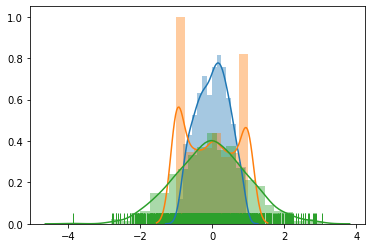
normal 분포의 경우 sampling을 했을 때 특정 구간을 벗어나는 경우가 발생한다.
이 경우를 처리하기 위해서 cliping을 하면 다음과 같이 깁스현상이 발생하고 많은 경우에 문제가 발생한다.
따라서 위의 경우에는 beta 분포를 사용하여 완화할 수 있다.
Numerical KL divergence of gaussian distribution
\(\begin{align} D_{KL}(p||q) &= -\int p(x)\log{\frac{p(x)}{q(x)}} \\ &= \log{\frac{\sigma_2}{\sigma_1}} + \frac{\sigma_1^2 + (\mu_1 - \mu_2)^2}{2\sigma_2^2} - \frac{1}{2}\\ \end{align}\) when 1st distribution is standard normal, $\mu_1 = 0,\sigma_1 = 1$
\[\begin{align} D_{KL}(p=N(0,1)||q) & \approx \frac{1}{2n}\sum_{i=1}^n(\frac{\mu_{2i}^2 + 1}{\sigma_{2i}^2} + \log\sigma_{2i}^2 - 1) \end{align}\]when 2nd distribution is standard normal, $\mu_2 = 0,\sigma_2 = 1$ \(\begin{align} D_{KL}(p||q=N(0,1)) & \approx \frac{1}{2n}\sum_{i=1}^n(\mu_{1i}^2 + \sigma_{1i}^2 - \log\sigma_{1i}^2 - 1) \end{align}\)
1
2
3
4
5
6
7
8
9
10
11
12
13
14
def gauss_kld(mu_dist = 0., sig_dist = 0., n_sample=100, is_reverse = True):
    mu = torch.zeros(size=(n_sample,1),dtype=float)
    sigma = torch.ones(size=(n_sample,1),dtype=float)
    st_normal = torch.distributions.Normal(mu,sigma)

    mu = mu + mu_dist
    sigma = sigma + sig_dist
    normal = torch.distributions.Normal(mu,sigma)

    if is_reverse:
        kld = 0.5 * torch.sum((mu ** 2) + (sigma ** 2) - torch.log((sigma ** 2) + 1e-6) - 1, dim=1) # reverse - mode seeking
    else:
        kld = 0.5 * torch.sum(((mu ** 2) + 1 )/(sigma ** 2) + torch.log((sigma ** 2) + 1e-6) - 1, dim=1) # forward - mean seeking
    return torch.mean(kld), st_normal, normal
1
2
3
4
5
6
7
8
9
10
11
12
13
14
15
16
17
18
19
20
21
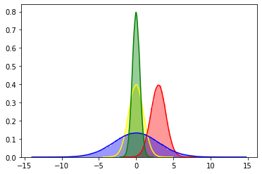
print("in reverse case")
kld, st_normal, normal = gauss_kld(3, 0)
print("bias kl divergence : ",kld.item())
x = [st_normal.sample().numpy() for _ in range(1000)]
y = [normal.sample().numpy() for _ in range(1000)]
# more stochastic
kld, st_normal, normal = gauss_kld(0, 2)
print("stochastic kl divergence : ",kld.item())
z = [normal.sample().numpy() for _ in range(1000)]
# more deterimistic
kld, st_normal, normal = gauss_kld(0, -0.5)
print("deterimistic kl divergence : ",kld.item())
w = [normal.sample().numpy() for _ in range(1000)]
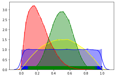
sns.distplot(x, color='yellow')
sns.distplot(y, color='red', label='bias')
sns.distplot(z, color='blue', label='stochastic')
sns.distplot(w, color='green', label='deterimistic')
# sns.jointplot(x,y, kind="kde")
1
2
3
4
5
in reverse case
bias kl divergence :  4.499999500000249
stochastic kl divergence :  2.901387655776337
deterimistic kl divergence :  0.3181451805639454
1
<matplotlib.axes._subplots.AxesSubplot at 0x7fbb24daa320>
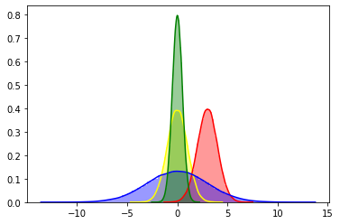
정규분포의 경우 알고 있듯이
mean을 바꾸면 bias가 달라지고
variance를 바꾸면 결정적인 정도가 바뀐다.
bias를 바꾸면 당연히 kl divergence가 증가 하겠지만
초록색과 파랑색처럼 결정적인 정도를 가지고 두 분포를 비교할 때 문제가 발생한다.
역방향 kl divergence는 mode seeking이므로
노랑색이 0인 부분에서 파랑색이 존재한다면 큰 panalty를 부여한다.
그래서 아래의 그래프를 보자.
1
2
3
4
5
6
7
8
9
10
11
12
13
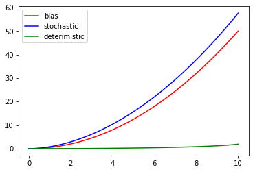
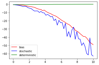
dist_list = np.linspace(0,10,num=50)
kld_list = [gauss_kld(x)[0] for x in dist_list]
plt.plot(dist_list, kld_list, color='red', label='bias')
# more stochastic
kld_list = [gauss_kld(0,x)[0] for x in dist_list]
plt.plot(dist_list, kld_list, color='blue', label='stochastic')
# more deterimistic
kld_list = [gauss_kld(0,-x/11)[0] for x in dist_list]
plt.plot(dist_list, kld_list, color='green', label='deterimistic')
plt.legend()
1
<matplotlib.legend.Legend at 0x7fbb22a5e2e8>
1
2
3
4
5
6
7
8
9
10
11
12
13
dist_list = np.linspace(0,10,num=50)
kld_list = [gauss_kld(x, is_reverse=False)[0] for x in dist_list]
plt.plot(dist_list, kld_list, color='red', label='bias')

# more stochastic
kld_list = [gauss_kld(0,x, is_reverse=False)[0] for x in dist_list]
plt.plot(dist_list, kld_list, color='blue', label='stochastic')

# more deterimistic
kld_list = [gauss_kld(0,-x/11, is_reverse=False)[0] for x in dist_list]
plt.plot(dist_list, kld_list, color='green', label='deterimistic')

plt.legend()
1
<matplotlib.legend.Legend at 0x7fbb22a2ed30>
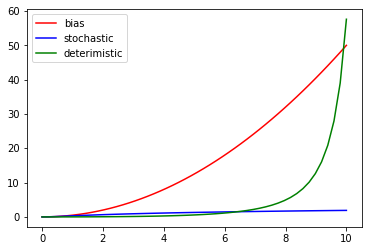
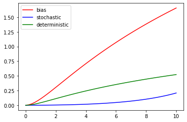
위의 그래프에서 보이듯이
forward kl divergence 사용했을 때
파란색 그래프를 보면 점점 stochasitic 해져도 값이 증가하지 않는다.
하지만 초록색 그래프를 보면 점점 deterministic해지는 경우 급격히 값이 증가한다.
즉, stochastic 한 경우 값이 작아지게 된다.
따라서 분포를 deterministic하게 만드는 파라미터를 찾고자 할 때
forward kl divergence를 사용하면 불리하게 작용할 수 있다.
Numerical loglikelihood of gaussian distribution
\(\begin{align} \sum_{i=1}^{n}\ln f(x_i | \mu, \sigma^2) &= -\frac{1}{2}(n\ln{2\pi} + n\ln{\sigma^2} + \sum_{i=1}^{n}\frac{(x_i - \mu)^2}{\sigma^2}) \\ & \approx -\frac{1}{2n}\sum_{i=1}^{n}(\ln{\sigma_i^2} + \frac{x_i - \mu_i}{\sigma_i^2}) \end{align}\)
보통 loglikelihood는 관측값만 있을때
그 관측값을 사용해서 특정 분포라는 가정을 하고
그분포의 파라미터를 찾아내는 방법이다.
이어서 loglikelihood의 값이 분포의 결정적인 정도에 따라서 어떻게 달라지나 보자.
1
2
3
4
5
6
7
8
9
def gauss_loglike(mu_dist = 0, sig_dist = 0, n_sample=100):
    mus = torch.zeros(size=(n_sample,1),dtype=float)
    sigmas = torch.ones(size=(n_sample,1),dtype=float)
    p_normal = torch.distributions.Normal(mus, sigmas)
    a_normal = torch.distributions.Normal(mus + mu_dist, sigmas + sig_dist)
    actions = a_normal.sample()
    log_likelihood = -torch.mean(0.5 * torch.log(sigmas.pow(2)) + \
                        ((actions - mus).pow(2)/(2.0*sigmas.pow(2))))
    return log_likelihood, p_normal, a_normal
1
2
3
4
5
6
7
8
9
10
11
12
13
14
15
16
17
18
log_likelihood, poicy_normal, action_normal = gauss_loglike(3,0)
x = [poicy_normal.sample().numpy() for _ in range(1000)]
y = [action_normal.sample().numpy() for _ in range(1000)]
print("bias log_likelihood: ",log_likelihood.item())

log_likelihood, poicy_normal, action_normal = gauss_loglike(0,2)
z = [action_normal.sample().numpy() for _ in range(1000)]
print("stochastic log_likelihood: ",log_likelihood.item())

log_likelihood, poicy_normal, action_normal = gauss_loglike(0,-0.5)
w = [action_normal.sample().numpy() for _ in range(1000)]
print("deterministic log_likelihood: ",log_likelihood.item())

sns.distplot(x, color="yellow")
sns.distplot(y, color="red")
sns.distplot(z, color="blue")
sns.distplot(w, color="green")
# sns.jointplot(x,y, kind="kde")
1
2
3
4
bias log_likelihood:  -4.899941049401496
stochastic log_likelihood:  -4.236859793801894
deterministic log_likelihood:  -0.09977808932281436
1
<matplotlib.axes._subplots.AxesSubplot at 0x7fbb229ba588>
1
2
3
4
5
6
7
8
9
10
11
12
13
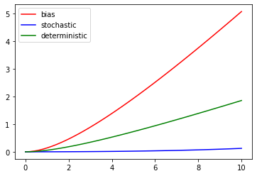
dist_list = np.linspace(0,10,num=50)
loglike_list = [gauss_loglike(x)[0] for x in dist_list]
plt.plot(dist_list, loglike_list, color='red', label='bias')
# more stochastic
loglike_list = [gauss_loglike(0,x)[0] for x in dist_list]
plt.plot(dist_list, loglike_list, color='blue', label='stochastic')
# more deterministic
dist_list = np.linspace(0,10,num=50)
loglike_list = [gauss_loglike(0,-x/11)[0] for x in dist_list]
plt.plot(dist_list, loglike_list, color='green', label='deterministic')
plt.legend()
1
<matplotlib.legend.Legend at 0x7fbb226e1d30>
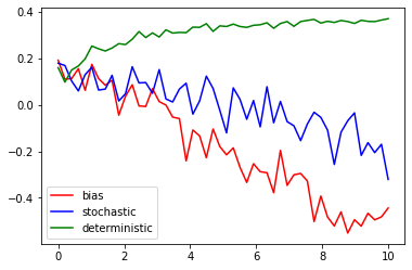
위의 그래프에서 보이듯이 logliklihood의 그래프 특성이
kl disvergence의 reverse방향과 유사하다는 것을 알 수 있다.
결국 logliklihood를 최대화 하는 방향의 파라미터를 찾다보면
추종하는 파라미터를 결정적으로 얻을 수 있게 된다.
Beta distribution
beta function은 다들 익숙하지 않아서 이론적 배경은 간략하게 나마 설명하고 간다.
pdf of beta distribution
\(\begin{align} f(x;\alpha,\beta) &= \frac{\Gamma(\alpha + \beta)}{\Gamma(\alpha)\Gamma(\beta)} x^{\alpha -1}(1-x)^{\beta-1} \\ &= \frac{1}{B(\alpha,\beta)}x^{\alpha -1}(1-x)^{\beta-1} \end{align}\)
beta function
여기서 beta function은 normalization constant를 의미한다. \(\begin{align} B(\alpha,\beta) = \frac{\Gamma(\alpha)\Gamma(\beta)}{\Gamma(\alpha + \beta)} \end{align}\)
disgamma function
그리고 digamma function은 gamma function에 대한 logarithmatic derivative로
계산적 용이성을 위해서 정의한 함수이다.
wikipedia를 참고바란다.
\(\begin{align}
\psi(\alpha) = \frac{d\ln{\Gamma(\alpha)}}{d\alpha}
\end{align}\)
Numerical KL divergence of beta distribution
\(\begin{align} D_{KL}(X_1 || X_2) &= \int_0^1 f(x;\alpha_1,\beta_1) \ln(\frac{f(x;\alpha_1,\beta_1)}{f(x;\alpha_2,\beta_2)}) dx \\ &= \ln(\frac{B(\alpha_2,\beta_2)}{B(\alpha_1,\beta_1)} + (\alpha_1 - \alpha_2) \psi(\alpha_1) + (\beta_1 - \beta_2) \psi(\beta_1) + (\alpha_2 - \alpha_1 + \beta_2 - \beta_1)\psi(\alpha_1 + \beta_1)\\ &= \ln(\frac{B(\alpha_2,\beta_2)}{B(\alpha_1,\beta_1)} + (\alpha_1 - \alpha_2) \psi(\alpha_1)+ (\beta_1 - \beta_2) \psi(\beta_1)+ (\alpha_2 - \alpha_1 + \beta_2 - \beta_1)\psi(\alpha_1 + \beta_1)\\ \end{align}\)
\[\therefore D_{KL}(X_1 || X_2) \approx \frac{1}{n}\sum_{i-1}^{n}[ \ln(\frac{B(\alpha_{2i},\beta_{2i})}{B(\alpha_{1i},\beta_{1i})}) + (\alpha_{1i} - \alpha_{2i}) \psi(\alpha_{1i})+ (\beta_{1i} - \beta_{2i}) \psi(\beta_{1i})+ (\alpha_{2i} - \alpha_{1i} + \beta_{2i} - \beta_{1i})\psi(\alpha_{1i} + \beta_{1i})]\]1
2
3
4
5
6
7
8
9
10
11
12
13
14
15
16
17
18
19
20
21
22
23
24
def beta_function(a,b):
beta =(torch.lgamma(a).exp()*torch.lgamma(b).exp())/(torch.lgamma(a + b).exp())
return beta
def beta_kld(a_dist = 0., b_dist = 0., a_base = 2, b_base = 2, n_sample = 100, is_forward=True):
if is_forward is True:
a1 = torch.zeros(size=(n_sample,1),dtype=float) + a_base
b1 = torch.zeros(size=(n_sample,1),dtype=float) + b_base
st_beta = torch.distributions.Beta(a1,b1)
a2 = a1 + a_dist
b2 = b1 + b_dist
beta = torch.distributions.Beta(a2, b2)
else:
a2 = torch.zeros(size=(n_sample,1),dtype=float) + a_base
b2 = torch.zeros(size=(n_sample,1),dtype=float) + b_base
st_beta = torch.distributions.Beta(a2,b2)
a1 = a2 + a_dist
b1 = b2 + b_dist
beta = torch.distributions.Beta(a2, b2)
kld = torch.log(beta_function(a2,b2)/beta_function(a1,b1))
kld += (a1-a2)*torch.digamma(a1)
kld += (b1-b2)*torch.digamma(b1)
kld += (a2 - a1 + b2 - b1)*torch.digamma(a1 + b1)
return torch.mean(kld), st_beta, beta
beta 분포의 kl divergence는 $\alpha \neq \beta$인 skewed case 에 대해서 대칭성을 지닌다.
1
2
3
4
print(beta_kld(1, 1)[0]) # 알파1 = 3, 베타1 = 3, 알파1 = 2, 베타1 = 2
print(beta_kld(1, 1, is_forward=False)[0]) # 알파1 = 2, 베타1 = 2, 알파1 = 3, 베타1 = 3
print(beta_kld(-2.5, 2.5, 3, 0.5)[0]) # 알파1 = 3, 베타1 = 0.5, 알파1 = 0.5, 베타1 = 3
print(beta_kld(-2.5, 2.5, 3, 0.5, is_forward=False)[0]) # 알파1 = 3, 베타1 = 0.5, 알파1 = 0.5, 베타1 = 3
1
2
3
4
5
tensor(0.0572, dtype=torch.float64)
tensor(0.0428, dtype=torch.float64)
tensor(7.2157, dtype=torch.float64)
tensor(7.2157, dtype=torch.float64)
1
2
3
4
5
6
7
8
9
10
11
12
13
14
15
16
17
18
19
20
kld, st_beta, beta = beta_kld(5, 0)
print("bias kl divergence : ",kld.item())
x = [st_beta.sample().numpy() for _ in range(1000)]
y = [beta.sample().numpy() for _ in range(1000)]

# more stochastic
kld, st_beta, beta = beta_kld(-1, -1)
print("stochastic kl divergence : ",kld.item())
z = [beta.sample().numpy() for _ in range(1000)]

# more deterministic
kld, st_beta, beta = beta_kld(5, 5)
print("deterministic kl divergence : ",kld.item())
w = [beta.sample().numpy() for _ in range(1000)]

sns.distplot(x,rug=True,color='yellow')
sns.distplot(y,rug=True,color='red')
sns.distplot(z,rug=True,color='blue')
sns.distplot(w,rug=True,color='green')
# sns.jointplot(x,y, kind="kde")
1
2
3
4
bias kl divergence :  1.9330744451595712
stochastic kl divergence :  0.12509280256138844
deterministic kl divergence :  0.731431373458168
1
<matplotlib.axes._subplots.AxesSubplot at 0x7fbb226a36a0>
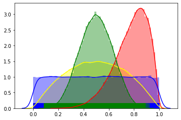
그래프를 보면 normal 분포와 확연히 다른 부분이 있다.
- kl divergence그래프가 순방향 역방향 스케일만 다를 뿐 비슷산 양상을 보인다.
- 순방향 역방향 모두 stochastic 할 때 값이 더 작다.
- normal 분포의 kl divergence 와 비교하여 값의 스케일이 약 10배 정도 차이난다.
3번의 특징 때문에 만약 normal 분포의 kl divergence로 loss function을 만들었던 부분을
beta 분포의 kl divergence로 바꾼다면 상수를 10배정도 늘려 주는 것이 좋을 것으로 예상된다.
1
2
3
4
5
6
7
8
9
10
dist_list = np.linspace(0,10,num=50)
kld_list = [beta_kld(x)[0] for x in dist_list]
plt.plot(dist_list, kld_list, color='red', label='bias') # bias

kld_list = [beta_kld(-x/10, -x/10)[0] for x in dist_list]
plt.plot(dist_list, kld_list, color='blue', label='stochastic') # more stochastic

kld_list = [beta_kld(x,x)[0] for x in dist_list]
plt.plot(dist_list, kld_list, color='green', label='deterministic') # more deterministic
plt.legend()
1
<matplotlib.legend.Legend at 0x7fbb22984f28>
1
2
3
4
5
6
7
8
9
10
dist_list = np.linspace(0,10,num=50)
kld_list = [beta_kld(x, is_forward = False)[0] for x in dist_list]
plt.plot(dist_list, kld_list, color='red', label='bias') # bias

kld_list = [beta_kld(-x/10,-x/10, is_forward = False)[0] for x in dist_list]
plt.plot(dist_list, kld_list, color='blue', label='stochastic') # more stochastic

kld_list = [beta_kld(x,x, is_forward = False)[0] for x in dist_list]
plt.plot(dist_list, kld_list, color='green', label='deterministic') # more deterministic
plt.legend()
1
<matplotlib.legend.Legend at 0x7fbb24cf00b8>
Numerical loglikelihood of beta distribution
\(\begin{align} \sum_{i=1}^{n}\ln{f(X_i|\alpha, \beta)} &= (\alpha - 1) \sum_{i=1}^{n}\ln{x_i}+ (\beta- 1) \sum_{i=1}^{n}\ln{(1 - x_i)}- n\ln{B(\alpha, \beta)}\\ &= \frac{1}{n}\sum_{i=1}^{n} [(\alpha_i - 1)\ln{x_i}+ (\beta_i- 1) \ln{(1 - x_i)}- \ln{B(\alpha_i, \beta_i)}] \end{align}\)
1
2
3
4
5
6
7
8
9
10
def beta_loglike(a_dist = 0., b_dist = 0., n_sample = 100):
    a1 = torch.ones(size=(n_sample,1),dtype=float) + 1
    b1 = torch.ones(size=(n_sample,1),dtype=float) + 1
    p_beta = torch.distributions.Beta(a1, b1)
    a_beta = torch.distributions.Beta(a1 + a_dist, b1 + b_dist)
    actions = a_beta.sample()
    log_likelihood = (a1 - 1)*torch.log(actions + 1e-6)
    log_likelihood += (b1 - 1)*torch.log(1 - actions + 1e-6)
    log_likelihood -= torch.log(beta_function(a1,b1))
    return torch.mean(log_likelihood), p_beta, a_beta
1
2
3
4
5
6
7
8
9
10
11
12
13
14
15
16
17
18
19
20
log_likelihood, poicy_beta, action_beta = beta_loglike(0,5)
x = [poicy_beta.sample().numpy() for _ in range(1000)]
y = [action_beta.sample().numpy() for _ in range(1000)]
print("bias log_likelihood: ",log_likelihood.item())

# more stochastic
log_likelihood, poicy_beta, action_beta = beta_loglike(-1,-1)
z = [action_beta.sample().numpy() for _ in range(1000)]
print("stochastic log_likelihood: ",log_likelihood.item())

# more deterministic
log_likelihood, poicy_beta, action_beta = beta_loglike(5,5)
w = [action_beta.sample().numpy() for _ in range(1000)]
print("deterministic log_likelihood: ",log_likelihood.item())

sns.distplot(x,rug=True, color="yellow")
sns.distplot(y,rug=True, color="red")
sns.distplot(z,rug=True, color="blue")
sns.distplot(w,rug=True, color="green")
# sns.jointplot(x,y, kind="kde")
1
2
3
4
bias log_likelihood:  -0.12187728064832459
stochastic log_likelihood:  -0.3756179701300583
deterministic log_likelihood:  0.33329267158708764
1
<matplotlib.axes._subplots.AxesSubplot at 0x7fbb24dd4080>
1
2
3
4
5
6
7
8
9
10
11
12
13
14
dist_list = np.linspace(0,10,num=50)
loglike_list = [beta_loglike(x)[0] for x in dist_list]
plt.plot(dist_list, loglike_list, color='red', label='bias')

# more stochastic
dist_list = np.linspace(0,10,num=50)
loglike_list = [beta_loglike(-x/10,-x/10)[0] for x in dist_list]
plt.plot(dist_list, loglike_list, color='blue', label='stochastic')

# more deterministic
dist_list = np.linspace(0,10,num=50)
loglike_list = [beta_loglike(x,x)[0] for x in dist_list]
plt.plot(dist_list, loglike_list, color='green', label='deterministic')
plt.legend()
1
<matplotlib.legend.Legend at 0x7fbaf2d66c18>
위의 그래프에서 보이듯이 logliklihood의 그래프 특성이
kl disvergence의 logliklihood와 유사하다는 것을 알 수 있다.
따라서 마찬가지로 베타분포도 결국 logliklihood를 최대화 하는 방향의 파라미터를 찾다보면
추종하는 파라미터를 결정적으로 얻을 수 있게 된다.
하지만 스케일이 10배정도 작으므로 앞에 상수를 normal 분포의 10배정도로 설정하는 것이 좋을 것으로 예상된다.
베타분포의 파라미터에 대한 변화를 살펴보자
1
2
3
4
5
6
7
import numpy as np
import torch

import matplotlib.pyplot as plt
# from celluloid import Camera

import seaborn as sns
1
2
from IPython.display import HTML
from matplotlib.animation import FuncAnimation
1
2
3
4
5
6
7
8
9
10
11
12
13
14
15
16
17
18
19
20
21
frames = torch.from_numpy(np.arange(2., 5, 0.1)).type(torch.FloatTensor)
f, axes =  plt.subplots()
color=['red','blue']

def animation(i):
    plt.cla()
    for j in range(2):
        if j == 0:
            beta = torch.distributions.Beta(i,torch.tensor(2.))
        else:
            beta = torch.distributions.Beta(torch.tensor(2.),i)
        x = [beta.sample().numpy() for _ in range(10**4)]
        sns.distplot(x,color=color[j])


ani = FuncAnimation(
        fig=f, func=animation,
        frames=frames,
        blit=False) # True일 경우 update function에서 artist object를 반환해야 함

HTML(ani.to_html5_video())

Leave a comment