
Interior Point Method
Large scale 에서 non-linear programing 방법으로 많이 사용되는 Ipopt(Interior point optimization) 혹은 barrier method라고 불리는 방법 에 대해서 알아보자.
Overview
nonlinear constraint optimization을 풀기 위해서 equality constraint에 log barrrier function을 도입하여 lagrange dual problem으로 바꾸는 과정을 알아본다.
이후 Ipopt pseudo code를 보고 구현해서 예제를 구현해보자.
1
2
3
4
5
6
7
8
9
10
import numpy as np
np.set_printoptions(precision=2, suppress=True)
from matplotlib import pyplot as plt
from copy import deepcopy
import matplotlib.cm as cm
from mpl_toolkits import mplot3d
import warnings
# warnings.filterwarnings(action='ignore')
import pdb
%matplotlib inline
Constraint Minimization
\(\underset{x}{min}f_{0}(x) \\ s.t \;\; f_{i}(x) \leq 0 \;\;,i=1,\dots,m \\ Ax = b\) 우선 optimization을 위의 형식으로 바꾸어야 되는 과정이 필요하다.
Logarithmic barrier funtion
\(\phi(x) = - \sum_{i=1}^{m} \log (- f_{i}(x)) \;\; ,dom \;\phi = \{ x | f_{i} (x) < 0, \;\; i=1,\dots,m \}\)
1
2
3
4
5
6
7
8
def barrier(f, x, max_penelty=1000):
    '''
    f: m dimensional function call instance
    x: n dimensional variables
    '''
    penalty = -np.sum(np.log(-f(x)), axis=0)
#     penalty[np.isnan(penalty)] = max_penelty
    return penalty
1
2
3
4
5
6
7
8
9
from numpy import errstate

for t in [0.5, 1, 2, 10]:
    plt.plot(np.arange(-3, 1, 0.01), (1/t)*barrier(lambda x: np.array([x]), np.arange(-3, 1, 0.01)), label='t={}'.format(t))
plt.gca().set_xlim(-3,1)
plt.gca().set_ylim(-3,10)
plt.hlines(y=0, xmin=-3, xmax=0, linestyles='dotted', color = 'k')
plt.vlines(x=0, ymin=0, ymax=10, linestyles='dotted', color = 'k')
plt.legend()
1
2
3
4
5
6
7
8
9
/home/swyoo/anaconda3/envs/cvxpy/lib/python3.6/site-packages/ipykernel_launcher.py:6: RuntimeWarning: invalid value encountered in log

/home/swyoo/anaconda3/envs/cvxpy/lib/python3.6/site-packages/ipykernel_launcher.py:6: RuntimeWarning: invalid value encountered in log

/home/swyoo/anaconda3/envs/cvxpy/lib/python3.6/site-packages/ipykernel_launcher.py:6: RuntimeWarning: invalid value encountered in log

/home/swyoo/anaconda3/envs/cvxpy/lib/python3.6/site-packages/ipykernel_launcher.py:6: RuntimeWarning: invalid value encountered in log
1
<matplotlib.legend.Legend at 0x7f3921d38898>
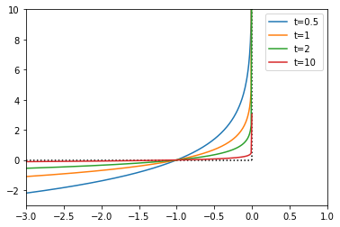
$f(x)=x$ 일경우 위의 예제를 보면 t 가 증가할수록 이상적인 penalty function과 가까워진다는 것을 알수 있다.
barrier function을 사용하면 standard Constraint Minimization 문제를 다음과 같이 inequality constraint를 penalty로 더하여 표현할 수 있다.
간단한 예제를 통해서 penalty가 추가되므로써 objective 가 어떻게 바뀌는지 알아보자. \(\underset{x \in \mathbb{R}}{min} \; (x+1)^2 \;\;s.t. \; x \geq 0\) standard constraint minimization 형태로 바꿀 수 있고 아래와 같다. \(\underset{x \in \mathbb{R}}{min} \; (x+1)^2 \;\;s.t. \; -x \leq 0\) 이때 objective와 constraint 함수는 아래와 같다. \(f_{0}(x) = (x+1)^2 \\ f_{1}(x) = -x\) log-barrier penalty를 더하여 unconstraint optimization으로 바꾸면 아래와 같다. \(\underset{x \in \mathbb{R}}{min} \; (x+1)^2 - \frac{1}{t} \ln x\)
1
2
3
4
5
6
7
8
9
10
11
12
13
14
f0 = lambda x: (x+1)**2
f1 = lambda x: np.array([-x])

x = np.arange(-2, 3, 0.01)
plt.plot(x, f0(x), label='Unconstraint')
for t in [0.5, 1, 2, 10]:
    plt.plot(x, f0(x) + (1/t)*barrier(f1, x), label='t={}'.format(t))

plt.gca().set_xlim(x.min(),x.max())
plt.gca().set_ylim(-1,10)
plt.hlines(y=0, xmin=x.min(), xmax=x.max(), linestyles='dotted', color = 'k')
plt.vlines(x=0, ymin=0, ymax=10, linestyles='dotted', color = 'k')
plt.legend()
1
2
3
4
5
6
7
8
9
/home/swyoo/anaconda3/envs/cvxpy/lib/python3.6/site-packages/ipykernel_launcher.py:6: RuntimeWarning: invalid value encountered in log

/home/swyoo/anaconda3/envs/cvxpy/lib/python3.6/site-packages/ipykernel_launcher.py:6: RuntimeWarning: invalid value encountered in log

/home/swyoo/anaconda3/envs/cvxpy/lib/python3.6/site-packages/ipykernel_launcher.py:6: RuntimeWarning: invalid value encountered in log

/home/swyoo/anaconda3/envs/cvxpy/lib/python3.6/site-packages/ipykernel_launcher.py:6: RuntimeWarning: invalid value encountered in log
1
<matplotlib.legend.Legend at 0x7f3921c60f60>
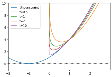
t 가 커질 수록 constraint가 강화되어서 feasible boundary쪽으로 optimal optimal point가 이동하는 것을 볼수있다.
다음과 같이 t에 따라 변하는 optimal point들의 집합을 central path라고 한다.
\(\{x^{*}(t)| t > 0\}\)
central path는 $f_{0}(x)$의 level curve를 따라서 이동한다.
Dual points on central path
모든 central point들은 그에 대응하는 dual feasible point들을 갖는다. 이때 duality gap이 t에 따라서 어떻게 달라지는 지 알아보자.
그것을 통해서 dual feasible point가 얼마만큼 sub-optimal한 값인지 알아보자.
central path $t > 0$ 에서 다음과 같은 문제의 해집합이다. \(\begin{align} \underset{x}{min} &\; f_{0}(x) - \frac{1}{t}\phi(x) \\ &s.t \;\; Ax = b \\ &,where \; \phi(x) = - \sum_{i=1}^{m} \log (- f_{i}(x)) \;\; ,dom \;\phi = \{ x | f_{i} (x) < 0, \;\; i=1,\dots,m \} \end{align}\)
위문제를 Lagrange dual prblem으로 바꾸기 위해서 KKT 조건 중 stationary condition에 의하면 다음과 같은 관계가 성립한다.
\[\begin{align} \nabla_{x} L(x, \nu^{*}) &= \nabla_{x} f_{0}(x) - \frac{1}{t} \nabla_{x} \phi(x) + \nabla (Ax-b)^{T}\nu^{*} \\ &= \nabla_{x} f_{0}(x) - \sum_{i=1}^{m} \frac{1}{t f_{i} (x)} \nabla_{x} f_{i} (x) + A^{T} \nu^{*} \\ \nabla_{x} \big[L(x, \nu^{*})\big]|_{x=x^{*}} &= \nabla_{x} f_{0}(x^{*}) - \sum_{i=1}^{m} \frac{1}{t f_{i} (x^{*})} \nabla_{x} f_{i} (x^{*}) + A^{T} \nu^{*} = 0 \end{align}\]위의 식을 다시 matrix form으로 정리하면 다음과 같다. \(\begin{align} \nabla_{x} f_{0}(x^{*}) + \nabla_{x} \lambda^{*}(t)^{T} F^{*} + A^{T} \nu^{*} &= 0 \\ \;\;,where \;F^{*} &= (f_{1}(x^{*}), \dots, f_{m}(x^{*})) \\ \lambda^{*}(t) &= (\lambda_{1}^{*}(t), \dots, \lambda_{m}^{*}(t)) ,\; \lambda_{i}^{*}(t) = \frac{1}{t f_{i} (x^{*})} \end{align}\)
따라서 Lagrange funtion은 다음과 같다.
\[L(x, \lambda, \nu) = f_{0}(x) + \lambda(t)^{T} F + \nu^{T}(Ax-b)\]기존 Lagrange funtion과 다른점은 complementary slackness가 다음과 같이 근사된다는 점이다. \(\lambda_{i} f_{i}(x) = 0 \rightarrow -\lambda_{i}(t) f_{i}(x) = \frac{1}{t} ,\; \forall i\)
이어서 Lagrange funtion 을 통해 구한 해가 얼마만큼 sub-optimal한 지를 살펴보자.
feasible 조건을 이용하면 아래와 같이 유도된다.
\(\begin{align}
p^{*} &\geq \underset{\lambda, \nu}{sup}\; L(x^{*}(t), \lambda(t), \nu) \\
&= f_{0}(x^{*}) - \sum_{i=1}^{m} \frac{1}{t f_{i} (x^{*})} f_{i} (x^{*}) + (Ax^{*}-b)^{T}\nu \\
&= f_{0}(x^{*}) - \frac{m}{t}
\end{align}\)
따라서 Ipopt 방법은 $\frac{m}{t} suboptimal$ 알고리즘이다.
Example
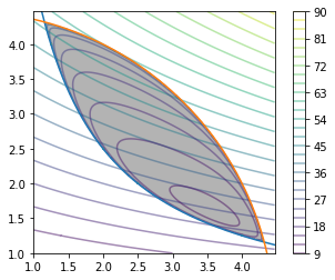
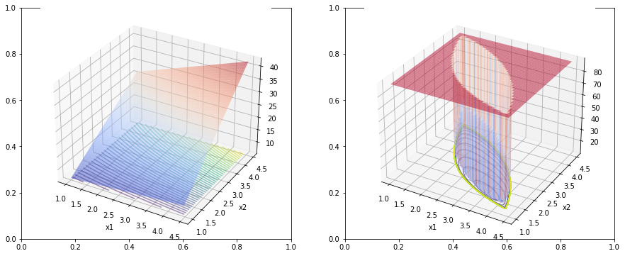
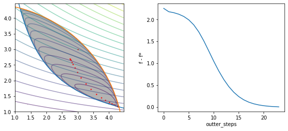
예제를 통해 다음과 같은 문제를 풀어보자 \(\begin{align} \underset{x\in \mathbb{R}^{2}}{min}\;& x_{2}(5 + x_{1}) \\ s.t. &\;\; x_1 x_2 \geq 5 \\ &x_{1}^{2} + x_{2}^{2} \leq 20 \end{align}\) 위의 식을 standard constraint minimization 식으로 바꾸면 다음과 같다. \(\begin{align} \underset{x\in \mathbb{R}^{2}}{min}\;& x_{2}(5 + x_{1}) \\ s.t. &\;\; 5-x_1 x_2 \leq 0 \\ &x_{1}^{2} + x_{2}^{2}-20 \leq 0 \end{align}\) 그러면 objective와 inequality constraint 는 다음과 같이 unconstraint optmization식으로 된다. \(\begin{align} \underset{x}{min} &\; f_{0}(x) - \frac{1}{t}\sum_{i=1}^{2} \log (- f_{i}(x)) \\ f_{0}(x) &= x_{2}(5 + x_{1})\\ f_{1}(x) &= 5-x_1 x_2\\ f_{2}(x) &= x_{1}^{2} + x_{2}^{2}-20\\ \end{align}\)
1
2
3
4
5
6
7
8
9
10
11
12
13
14
15
16
17
18
19
20
21
22
23
24
25
26
27
28
29
def f(x):
    return x[1]*(5+x[0])
def g(x):
    return (x[0]*x[1] >= 5) & (x[0]**2 + x[1]**2 <= 20)
def k(x):
    y1 = 5/x
    y2 = np.sqrt(20 - (x**2))
    return np.array([y1,y2])
def constr(x):
    f1 = 5 - x[0]*x[1]
    f2 = x[0]**2 + x[1]**2 - 20
    return np.array([f1,f2])

# plt.rcParams["figure.figsize"] = (5,5)
x = np.arange(1,np.sqrt(20),0.01)
plt.xlim(x.min(),x.max())
plt.ylim(x.min(),x.max())
plt.plot(x,k(x)[0])
plt.plot(x,k(x)[1])

x = np.array(np.meshgrid(x,x))
plt.imshow(g(x).astype(int) ,
           extent=(x[0].min(),x[0].max(),x[1].min(),x[1].max()),
           origin="lower", cmap="Greys", alpha = 0.3);
plt.contour(x[0],x[1],f(x), levels=20, alpha=0.5)
t = 0.5
plt.contour(x[0],x[1],f(x) + (1/t)*barrier(constr, x), levels=30, alpha=0.5)
plt.colorbar()
plt.show()
1
2
3
/home/swyoo/anaconda3/envs/cvxpy/lib/python3.6/site-packages/ipykernel_launcher.py:6: RuntimeWarning: invalid value encountered in log
pseudo-code
reference
given strictly feasible x, t := t(0) > 0, $\mu$ > 1, tolerance $\epsilon > 0$. repeat
- Centering step. Compute $x^{*}(t)$ by minimizing $tf_{0} + \phi$, subject to $Ax = b$.
- Update. x := $x^{*}(t)$.
- Stopping criterion. quit if $\frac{m}{t} < \epsilon$.
- Increase t. t := $\mu$t.
1
2
3
4
5
6
7
8
9
10
11
12
13
14
15
16
17
18
19
20
21
22
import matplotlib.cm as cm
x = np.arange(1,np.sqrt(20),0.01)
x = np.array(np.meshgrid(x,x))

fig, (ax1, ax2) = plt.subplots(nrows=1, ncols=2, figsize=(15, 6))
ax1 = fig.add_subplot(1, 2, 1, projection='3d')
ax1.set_xlabel('x1')
ax1.set_ylabel('x2')
y = f(x)
ax1.plot_surface(x[0], x[1], y, alpha=0.5, cmap='coolwarm')
ax1.contour(x[0], x[1], y, zdir='z', offset=y.min(), levels=50, alpha=0.5)

ax2 = fig.add_subplot(1, 2, 2, projection='3d')
ax2.set_xlabel('x1')
ax2.set_ylabel('x2')
t = 0.5
y = f(x) + (1/t)*barrier(constr, x)
y[np.isnan(y)] = y[~np.isnan(y)].max()
ax2.set_zlim(y[~np.isnan(y)].min()-1, y[~np.isnan(y)].max())
ax2.plot_surface(x[0], x[1], y, alpha=0.5, cmap='coolwarm')
ax2.contour(x[0], x[1], y, zdir='z', offset=y.min(), levels=50, alpha=0.5)
1
2
3
/home/swyoo/anaconda3/envs/cvxpy/lib/python3.6/site-packages/ipykernel_launcher.py:6: RuntimeWarning: invalid value encountered in log
1
<matplotlib.contour.QuadContourSet at 0x7f39212cda58>
1
2
3
4
5
6
7
8
9
10
11
12
13
14
15
16
17
18
19
20
21
22
23
24
25
26
27
28
29
30
31
32
33
34
35
36
37
38
39
40
41
42
43
44
45
46
47
48
49
50
51
52
53
54
55
56
57
58
59
60
61
62
63
64
65
66
67
68
69
70
71
72
73
74
75
76
77
78
79
80
81
82
83
84
85
86
87
88
89
90
91
92
93
94
95
96
97
98
99
100
101
102
103
104
105
106
107
108
109
110
111
112
113
114
115
116
117
118
119
120
121
122
123
124
125
126
127
128
129
130
131
132
133
134
135
136
137
138
139
140
141
142
143
144
145
146
def gradient(f, x, epsilon=1e-7, y=None):
    """ numerically find gradients.
    x: shape=[n] """
    grad = np.zeros_like(x, dtype=float)
    for i in range(len(x)):
        h = np.zeros_like(x, dtype=float)
        h[i] = epsilon
        if y is None:
            grad[i] = (f(x + h) - f(x - h)) / (2 * h[i])
        else:
            grad[i] = (f(x + h, y) - f(x - h, y)) / (2 * h[i])
    return grad

def grad_decent(f, init, step, y=None, lr=0.001, history=False):
    x = init
    memo = [x]
    for i in range(step):
        if y is None:
            grad = gradient(f, x)
        else:
            grad = gradient(f, x, y=y)
        x = x - lr * grad
        if history: memo.append(x)
    if not history: return x
    return x, np.array(list(zip(*memo)))

def jacobian(f, m, x, y=None, h=1e-7, verbose=False):
    """ numerically find jacobian, constraint: m > 1
    f: call instance with shape=[m]
    x: shape=[n] """
    n = len(x)
    jaco = np.zeros(shape=(m, n), dtype=float)
    for i in range(m):
        if y is None:
            jaco[i, :] = gradient(lambda e: f(e)[i], x)
        else:
            jaco[i, :] = gradient(lambda e, l: f(e, l)[i], x, y=y)
    if np.linalg.det(jaco) == 0:
        if verbose: print('jacobian is singular, use pseudo-inverse')
    return jaco

def raphson(f, m, init, nu=None, epsilon=1e-7, verbose=True, history=False, max_iter=1000):
    """ Newton Raphson Method.
    f: function
    m: the number of output dimension
    init: np.array, with dimension n """

    n = len(init)
    if nu is None:
        hessian = lambda f, n, x: jacobian(lambda e: gradient(f, e), n, x=x)
    else:
        hessian = lambda f, n, x, y: jacobian(lambda x, nu: gradient(f, x, y=nu), n, x=x, y=y)

    x = deepcopy(init)
    bound = 1e-7
    memo = [x]
    while max_iter:
        if nu is None:
            H_inv = np.linalg.inv(hessian(f, n=len(x), x=x))
            update = np.matmul(H_inv, gradient(f, x))
        else:
            H_inv = np.linalg.inv(hessian(f, n=len(x), x=x, y=nu))
            update = np.matmul(H_inv, gradient(f, x, y=nu))
        x = x - update
        if bound > sum(np.abs(update)):
            break
        if verbose: print("x={}, update={}".format(x, sum(np.abs(update))))
        if history: memo.append(x)
        max_iter -= 1
    if not history: return x
    return x, np.array(list(zip(*memo)))


def Ipopt(f, ieconstr, init, m, d_init=None, econstr=None, eps=1e-6, inner_step=100, mu=2, t=0.01, outter_step=10, verbose=True, inner_lr=0.01):
    t_values = []
    central_path = [init]
    ans = 0
    p_ans = 0
    if econstr is not None:
        d_central_path = [d_init]

    for i in range(outter_step):
        if m/t <= eps:
            print("finish!")
            break
        if econstr is None:
            objective = lambda e: t * f(e) + barrier(ieconstr, e)
            ans, history = raphson(objective, m=m, init=central_path[-1], verbose=False, history=True, max_iter=inner_step)
        else:
#             lagrange = lambda e,nu: t * f(e) + barrier(ieconstr, e) + np.dot(nu.T, econstr(e))

#             dual_function = lambda e: lagrange(grad_decent(lagrange, init=central_path[-1], y=e, step=inner_step, lr=0.01, history=False), e)
#             dual_function = lambda e: lagrange(raphson(lagrange, m=m, init=central_path[-1], nu=e, verbose=False, history=False, max_iter=inner_step), e)
#             objective = lambda e: -dual_function(e)

#             def objective(nu):
#                 nonlocal p_ans
#                 p_ans = grad_decent(lagrange, init=p_ans, y=nu, step=inner_step, lr=0.01, history=False)
#                 p_ans = grad_decent(lagrange, init=central_path[0], y=nu, step=inner_step, lr=0.01, history=False)
#                 p_ans = raphson(lagrange, m=m, init=central_path[-1], nu=nu, verbose=False, history=False, max_iter=inner_step) # it does not work in sigular case
#                 if True in np.isnan(p_ans):
#                     p_ans = central_path[0]
#                     return - lagrange(p_ans, nu)
#                 central_path.append(p_ans)
#                 return - lagrange(p_ans, nu)

#             ans, history = raphson(objective, m=m, init=d_central_path[-1], verbose=False, history=True, max_iter=inner_step) # it does not work in sigular case
#             ans, history = grad_decent(objective, init=d_central_path[-1], step=inner_step, lr=0.01, history=True)
#             ans = np.clip(ans, 0.1, 1000)

            lagrange = lambda e,nu: t * f(e) + barrier(ieconstr, e) + t * np.dot(nu.T, econstr(e))
            p_ans = grad_decent(lagrange, init=central_path[-1], y=d_central_path[-1], step=inner_step, lr=inner_lr, history=False)
#             p_ans = raphson(lagrange, m=m, init=central_path[-1], nu=d_central_path[-1], verbose=False, history=False, max_iter=inner_step)
            if True in np.isnan(p_ans):
                print("central point is nan so update is rejected into: {}".format(central_path[-1]))
                break
            else:
                central_path.append(p_ans)

            dual = lambda e: -lagrange(p_ans, e)
            ans = grad_decent(dual, init=d_central_path[-1], step=inner_step, lr=inner_lr, history=False)
#             ans = raphson(dual, m=m, init=d_central_path[-1], verbose=False, history=True, max_iter=inner_step)
#             ans = np.clip(ans, 0.01, 1000)

        if verbose:
            print("t: {}, ans: {}".format(t, ans))
            if econstr is not None:
                print("t: {}, p_ans: {}".format(t, p_ans))

        if econstr is None:
            if True in np.isnan(ans):
                print("central point is nan so update is rejected into: {}".format(central_path[-1]))
                break
            else:
                central_path.append(ans)
        else:
            if True in np.isnan(ans):
                print("d_central point is nan so update is rejected into: {}".format(d_central_path[-1]))
                break
            else:
                d_central_path.append(ans)

        t_values.append(t)
        t = mu * t

    return ans, np.array(central_path), np.array(t_values)
1
2
3
4
5
6
7
8
9
10
11
12
13
14
15
16
17
18
19
20
21
22
23
24
25
26
27
28
init = np.array([3,3])
ans, c_path, ts = Ipopt(f=f, ieconstr=constr, init=init, m=1, outter_step=100, inner_step=100,
                        mu=1.5, t=0.01, eps=0.01, verbose=True)

fig, (ax1, ax2) = plt.subplots(nrows=1, ncols=2, figsize=(10, 4))
fig.clf()
ax1 = fig.add_subplot(1, 2, 1)

x = np.arange(1,np.sqrt(20),0.01)
ax1.set_xlim(x.min(),x.max())
ax1.set_ylim(x.min(),x.max())
ax1.plot(x,k(x)[0])
ax1.plot(x,k(x)[1])

x = np.array(np.meshgrid(x,x))
ax1.imshow(g(x).astype(int),
           extent=(x[0].min(),x[0].max(),x[1].min(),x[1].max()),
           origin="lower", cmap="Greys", alpha = 0.3)
ax1.contour(x[0],x[1],f(x), levels=20, alpha=0.5)
ax1.scatter(c_path[:,0], c_path[:,1],s=2,color='r')
plt.contour(x[0],x[1],f(x) + barrier(constr, x), levels=30, alpha=0.5)

ax2 = fig.add_subplot(1, 2, 2)
order = list(range(len(c_path)))
gaps = [np.linalg.norm(p) for p in c_path - ans]
ax2.plot(order, gaps)
ax2.set_xlabel('outter_steps')
ax2.set_ylabel('f - f*')
1
2
3
4
5
6
7
8
9
10
11
12
13
14
15
16
17
18
19
20
21
22
23
24
25
t: 0.01, ans: [2.76 2.7 ]
t: 0.015, ans: [2.77 2.67]
t: 0.0225, ans: [2.79 2.64]
t: 0.03375, ans: [2.81 2.59]
t: 0.050625, ans: [2.85 2.52]
t: 0.0759375, ans: [2.91 2.41]
t: 0.11390625000000001, ans: [2.99 2.27]
t: 0.17085937500000004, ans: [3.11 2.09]
t: 0.25628906250000005, ans: [3.26 1.9 ]
t: 0.3844335937500001, ans: [3.42 1.72]
t: 0.5766503906250001, ans: [3.59 1.57]
t: 0.8649755859375001, ans: [3.75 1.45]
t: 1.2974633789062502, ans: [3.89 1.37]
t: 1.9461950683593754, ans: [4.01 1.3 ]
t: 2.919292602539063, ans: [4.09 1.26]
t: 4.378938903808595, ans: [4.16 1.23]
t: 6.568408355712892, ans: [4.21 1.2 ]
t: 9.852612533569339, ans: [4.25 1.19]
t: 14.778918800354008, ans: [4.27 1.18]
t: 22.168378200531013, ans: [4.29 1.17]
t: 33.25256730079652, ans: [4.3  1.17]
t: 49.87885095119478, ans: [4.3  1.16]
t: 74.81827642679217, ans: [4.31 1.16]
finish!
1
2
3
/home/swyoo/anaconda3/envs/cvxpy/lib/python3.6/site-packages/ipykernel_launcher.py:6: RuntimeWarning: invalid value encountered in log
1
Text(0, 0.5, 'f - f*')
1
2
3
4
5
6
7
8
9
10
11
12
13
14
15
16
17
18
19
20
21
22
23
24
25
26
27
28
29
30
31
32
33
34
35
36
37
38
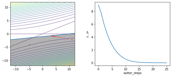
def f(x):
return x[1]**2 - 2*x[0]*x[1] + 4*x[1]**2
def constr(x):
f1 = -0.1*x[0] + x[1] + 1
return np.array([f1])
def g(x):
return -0.1*x[0] + x[1] + 1 <= 0
def k(x):
y = 0.1*x - 1
return y
init = np.array([-5,-4])
ans, c_path, ts = Ipopt(f=f, ieconstr=constr, init=init, m=2, outter_step=100, inner_step=100,
mu=1.5, t=0.01, eps=0.01, verbose=True)
fig, (ax1, ax2) = plt.subplots(nrows=1, ncols=2, figsize=(10, 4))
fig.clf()
ax1 = fig.add_subplot(1, 2, 1)
ax1.cla()
x = np.arange(-12,12,0.01)
ax1.set_xlim(x.min(),x.max())
ax1.set_ylim(x.min(),x.max())
ax1.plot(x,k(x))
x = np.array(np.meshgrid(x,x))
ax1.imshow(g(x).astype(int),
extent=(x[0].min(),x[0].max(),x[1].min(),x[1].max()),
origin="lower", cmap="Greys", alpha = 0.3)
ax1.contour(x[0],x[1],f(x), levels=20, alpha=0.5)
ax1.scatter(c_path[:,0], c_path[:,1],s=2,color='r')
ax2 = fig.add_subplot(1, 2, 2)
ax2.cla()
order = list(range(len(c_path)))
gaps = [np.linalg.norm(p) for p in c_path - ans]
ax2.plot(order, gaps)
ax2.set_xlabel('outter_steps')
ax2.set_ylabel('f - f*')
1
2
3
4
5
6
7
8
9
10
11
12
13
14
15
16
17
18
19
20
21
22
23
24
25
26
27
t: 0.01, ans: [10.95 -2.19]
t: 0.015, ans: [ 9.3  -1.86]
t: 0.0225, ans: [ 7.98 -1.6 ]
t: 0.03375, ans: [ 6.91 -1.38]
t: 0.050625, ans: [ 6.05 -1.21]
t: 0.0759375, ans: [ 5.37 -1.07]
t: 0.11390625000000001, ans: [ 4.84 -0.97]
t: 0.17085937500000004, ans: [ 4.43 -0.89]
t: 0.25628906250000005, ans: [ 4.12 -0.82]
t: 0.3844335937500001, ans: [ 3.89 -0.78]
t: 0.5766503906250001, ans: [ 3.72 -0.74]
t: 0.8649755859375001, ans: [ 3.6  -0.72]
t: 1.2974633789062502, ans: [ 3.52 -0.7 ]
t: 1.9461950683593754, ans: [ 3.46 -0.69]
t: 2.919292602539063, ans: [ 3.42 -0.68]
t: 4.378938903808595, ans: [ 3.39 -0.68]
t: 6.568408355712892, ans: [ 3.37 -0.67]
t: 9.852612533569339, ans: [ 3.36 -0.67]
t: 14.778918800354008, ans: [ 3.35 -0.67]
t: 22.168378200531013, ans: [ 3.34 -0.67]
t: 33.25256730079652, ans: [ 3.34 -0.67]
t: 49.87885095119478, ans: [ 3.34 -0.67]
t: 74.81827642679217, ans: [ 3.34 -0.67]
t: 112.22741464018824, ans: [ 3.34 -0.67]
t: 168.34112196028235, ans: [ 3.33 -0.67]
finish!
1
Text(0, 0.5, 'f - f*')
1
2
3
4
5
6
7
8
9
10
11
12
13
14
15
16
17
18
19
20
21
22
23
24
25
26
27
28
29
30
31
32
33
34
35
36
37
38
39
40
41
42
43
44
45
46
47
48
49
50
51
52
53
54
55
56
57
58
59
60
61
62
63
64
65
66
67
68
69
70
71
72
73
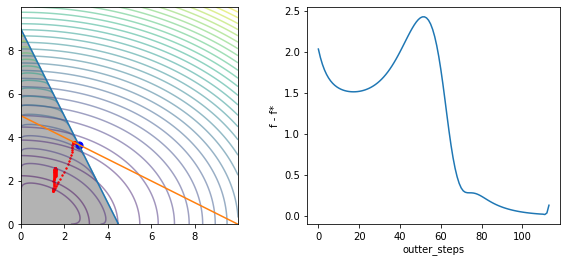
def f(x):
return (x[0]**2) + 2*(x[1]**2)
def ieconstr(x):
f1 = 2*x[0] + x[1] - 9
f2 = -x[0]
f3 = -x[1]
return np.array([f1,f2,f3])
def econstr(x):
f1 = x[0] + 2*x[1] - 10
return np.array([f1])
def g(x):
g1,g2,g3 = ieconstr(x)
return (g1 <= 0) & (g2 <= 0) & (g3 <= 0)
def k(x):
k1 = 9 - 2 * x
k2 = 5 - x / 2
return np.array([k1,k2])
import cvxpy as cp
x = cp.Variable(shape=(2))
cost = f(x)
constr = [2*x[0] +x[1]<= 9]
constr += [x[0] + 2 * x[1] == 10]
constr += [x[0] >= 0]
constr += [x[1] >= 0]
prob = cp.Problem(cp.Minimize(cost), constraints=constr)
prob.solve()
# Print result.
print("\nThe optimal cost is", prob.value)
optimal_point = x.value
print("The optimal point is", optimal_point)
init = np.array([1.5, 2])
d_init = np.array([1])
ans, c_path, ts = Ipopt(f=f, ieconstr=ieconstr, init=init, d_init=d_init, m=1,
econstr=econstr, outter_step=300, inner_step=4000,
mu=1.1, t=0.001, eps=0.01, verbose=True, inner_lr=0.0001)
print("answer is {}".format(c_path[-1]))
fig, (ax1, ax2) = plt.subplots(nrows=1, ncols=2, figsize=(10, 4))
fig.clf()
ax1 = fig.add_subplot(1, 2, 1)
ax1.cla()
x = np.arange(0,10,0.01)
ax1.set_xlim(x.min(),x.max())
ax1.set_ylim(x.min(),x.max())
ax1.plot(x,k(x)[0])
ax1.plot(x,k(x)[1])
x = np.array(np.meshgrid(x,x))
ax1.imshow(g(x).astype(int),
extent=(x[0].min(),x[0].max(),x[1].min(),x[1].max()),
origin="lower", cmap="Greys", alpha = 0.3)
ax1.contour(x[0],x[1],f(x), levels=30, alpha=0.5)
t = 1
ax1.contour(x[0],x[1], (t * f(x) + barrier(ieconstr, x) + t * d_init * econstr(x))[0] , levels=20, alpha=0.5)
ax1.scatter(c_path[:,0], c_path[:,1], s=2, color='r')
ax1.scatter(optimal_point[0], optimal_point[1], s=50, color='b')
ax2 = fig.add_subplot(1, 2, 2)
ax2.cla()
order = list(range(len(c_path)))
gaps = [np.linalg.norm(p) for p in c_path - optimal_point]
ax2.plot(order, gaps)
ax2.set_xlabel('outter_steps')
ax2.set_ylabel('f - f*')
1
2
3
4
5
6
7
8
9
10
11
12
13
14
15
16
17
18
19
20
21
22
23
24
25
26
27
28
29
30
31
32
33
34
35
36
37
38
39
40
41
42
43
44
45
46
47
48
49
50
51
52
53
54
55
56
57
58
59
60
61
62
63
64
65
66
67
68
69
70
71
72
73
74
75
76
77
78
79
80
81
82
83
84
85
86
87
88
89
90
91
92
93
94
95
96
97
98
99
100
101
102
103
104
105
106
107
108
109
110
111
112
113
114
115
116
117
118
119
120
121
122
123
124
125
126
127
128
129
130
131
132
133
134
135
136
137
138
139
140
141
142
143
144
145
146
147
148
149
150
151
152
153
154
155
156
157
158
159
160
161
162
163
164
165
166
167
168
169
170
171
172
173
174
175
176
177
178
179
180
181
182
183
184
185
186
187
188
189
190
191
192
193
194
195
196
197
198
199
200
201
202
203
204
205
206
207
208
209
210
211
212
213
214
215
216
217
218
219
220
221
222
223
224
225
226
227
228
229
230

The optimal cost is 33.999999999999986
The optimal point is [2.67 3.67]
t: 0.001, ans: [1.]
t: 0.001, p_ans: [1.55 2.09]
t: 0.0011, ans: [1.]
t: 0.0011, p_ans: [1.59 2.16]
t: 0.0012100000000000001, ans: [0.99]
t: 0.0012100000000000001, p_ans: [1.62 2.23]
t: 0.0013310000000000002, ans: [0.99]
t: 0.0013310000000000002, p_ans: [1.63 2.29]
t: 0.0014641000000000003, ans: [0.99]
t: 0.0014641000000000003, p_ans: [1.64 2.34]
t: 0.0016105100000000005, ans: [0.99]
t: 0.0016105100000000005, p_ans: [1.64 2.38]
t: 0.0017715610000000007, ans: [0.99]
t: 0.0017715610000000007, p_ans: [1.64 2.42]
t: 0.0019487171000000009, ans: [0.98]
t: 0.0019487171000000009, p_ans: [1.64 2.45]
t: 0.002143588810000001, ans: [0.98]
t: 0.002143588810000001, p_ans: [1.63 2.48]
t: 0.0023579476910000016, ans: [0.98]
t: 0.0023579476910000016, p_ans: [1.63 2.51]
t: 0.002593742460100002, ans: [0.97]
t: 0.002593742460100002, p_ans: [1.62 2.53]
t: 0.0028531167061100022, ans: [0.97]
t: 0.0028531167061100022, p_ans: [1.62 2.55]
t: 0.003138428376721003, ans: [0.97]
t: 0.003138428376721003, p_ans: [1.61 2.57]
t: 0.0034522712143931033, ans: [0.96]
t: 0.0034522712143931033, p_ans: [1.6  2.58]
t: 0.003797498335832414, ans: [0.96]
t: 0.003797498335832414, p_ans: [1.6  2.59]
t: 0.004177248169415656, ans: [0.95]
t: 0.004177248169415656, p_ans: [1.59 2.6 ]
t: 0.004594972986357222, ans: [0.94]
t: 0.004594972986357222, p_ans: [1.59 2.61]
t: 0.005054470284992944, ans: [0.94]
t: 0.005054470284992944, p_ans: [1.58 2.61]
t: 0.005559917313492239, ans: [0.93]
t: 0.005559917313492239, p_ans: [1.58 2.61]
t: 0.006115909044841464, ans: [0.92]
t: 0.006115909044841464, p_ans: [1.58 2.61]
t: 0.006727499949325611, ans: [0.91]
t: 0.006727499949325611, p_ans: [1.57 2.61]
t: 0.007400249944258173, ans: [0.91]
t: 0.007400249944258173, p_ans: [1.57 2.6 ]
t: 0.008140274938683991, ans: [0.89]
t: 0.008140274938683991, p_ans: [1.57 2.59]
t: 0.00895430243255239, ans: [0.88]
t: 0.00895430243255239, p_ans: [1.56 2.58]
t: 0.00984973267580763, ans: [0.87]
t: 0.00984973267580763, p_ans: [1.56 2.57]
t: 0.010834705943388393, ans: [0.86]
t: 0.010834705943388393, p_ans: [1.56 2.55]
t: 0.011918176537727233, ans: [0.84]
t: 0.011918176537727233, p_ans: [1.56 2.53]
t: 0.013109994191499958, ans: [0.82]
t: 0.013109994191499958, p_ans: [1.56 2.51]
t: 0.014420993610649954, ans: [0.8]
t: 0.014420993610649954, p_ans: [1.55 2.49]
t: 0.01586309297171495, ans: [0.78]
t: 0.01586309297171495, p_ans: [1.55 2.46]
t: 0.017449402268886447, ans: [0.75]
t: 0.017449402268886447, p_ans: [1.55 2.43]
t: 0.019194342495775094, ans: [0.73]
t: 0.019194342495775094, p_ans: [1.55 2.39]
t: 0.021113776745352607, ans: [0.69]
t: 0.021113776745352607, p_ans: [1.55 2.36]
t: 0.02322515441988787, ans: [0.66]
t: 0.02322515441988787, p_ans: [1.55 2.32]
t: 0.02554766986187666, ans: [0.62]
t: 0.02554766986187666, p_ans: [1.55 2.27]
t: 0.02810243684806433, ans: [0.57]
t: 0.02810243684806433, p_ans: [1.55 2.23]
t: 0.030912680532870763, ans: [0.52]
t: 0.030912680532870763, p_ans: [1.54 2.18]
t: 0.034003948586157844, ans: [0.47]
t: 0.034003948586157844, p_ans: [1.54 2.13]
t: 0.037404343444773634, ans: [0.4]
t: 0.037404343444773634, p_ans: [1.54 2.07]
t: 0.041144777789251, ans: [0.33]
t: 0.041144777789251, p_ans: [1.54 2.02]
t: 0.0452592555681761, ans: [0.25]
t: 0.0452592555681761, p_ans: [1.53 1.96]
t: 0.049785181124993715, ans: [0.15]
t: 0.049785181124993715, p_ans: [1.53 1.9 ]
t: 0.054763699237493094, ans: [0.05]
t: 0.054763699237493094, p_ans: [1.52 1.85]
t: 0.06024006916124241, ans: [-0.07]
t: 0.06024006916124241, p_ans: [1.52 1.79]
t: 0.06626407607736666, ans: [-0.2]
t: 0.06626407607736666, p_ans: [1.51 1.74]
t: 0.07289048368510333, ans: [-0.35]
t: 0.07289048368510333, p_ans: [1.51 1.69]
t: 0.08017953205361367, ans: [-0.52]
t: 0.08017953205361367, p_ans: [1.5  1.65]
t: 0.08819748525897504, ans: [-0.7]
t: 0.08819748525897504, p_ans: [1.5  1.61]
t: 0.09701723378487255, ans: [-0.91]
t: 0.09701723378487255, p_ans: [1.5  1.58]
t: 0.10671895716335981, ans: [-1.14]
t: 0.10671895716335981, p_ans: [1.49 1.55]
t: 0.1173908528796958, ans: [-1.4]
t: 0.1173908528796958, p_ans: [1.5  1.54]
t: 0.1291299381676654, ans: [-1.68]
t: 0.1291299381676654, p_ans: [1.5  1.54]
t: 0.14204293198443196, ans: [-1.98]
t: 0.14204293198443196, p_ans: [1.51 1.55]
t: 0.15624722518287518, ans: [-2.32]
t: 0.15624722518287518, p_ans: [1.53 1.57]
t: 0.1718719477011627, ans: [-2.68]
t: 0.1718719477011627, p_ans: [1.55 1.61]
t: 0.189059142471279, ans: [-3.06]
t: 0.189059142471279, p_ans: [1.58 1.67]
t: 0.20796505671840693, ans: [-3.47]
t: 0.20796505671840693, p_ans: [1.62 1.74]
t: 0.22876156239024764, ans: [-3.89]
t: 0.22876156239024764, p_ans: [1.67 1.84]
t: 0.2516377186292724, ans: [-4.33]
t: 0.2516377186292724, p_ans: [1.74 1.96]
t: 0.2768014904921997, ans: [-4.77]
t: 0.2768014904921997, p_ans: [1.81 2.1 ]
t: 0.3044816395414197, ans: [-5.21]
t: 0.3044816395414197, p_ans: [1.9  2.25]
t: 0.33492980349556173, ans: [-5.64]
t: 0.33492980349556173, p_ans: [1.99 2.42]
t: 0.36842278384511795, ans: [-6.04]
t: 0.36842278384511795, p_ans: [2.08 2.59]
t: 0.40526506222962977, ans: [-6.42]
t: 0.40526506222962977, p_ans: [2.17 2.76]
t: 0.44579156845259277, ans: [-6.76]
t: 0.44579156845259277, p_ans: [2.24 2.92]
t: 0.4903707252978521, ans: [-7.07]
t: 0.4903707252978521, p_ans: [2.29 3.07]
t: 0.5394077978276374, ans: [-7.34]
t: 0.5394077978276374, p_ans: [2.33 3.2 ]
t: 0.5933485776104012, ans: [-7.59]
t: 0.5933485776104012, p_ans: [2.35 3.31]
t: 0.6526834353714414, ans: [-7.8]
t: 0.6526834353714414, p_ans: [2.36 3.42]
t: 0.7179517789085855, ans: [-7.97]
t: 0.7179517789085855, p_ans: [2.37 3.5 ]
t: 0.7897469567994442, ans: [-8.12]
t: 0.7897469567994442, p_ans: [2.38 3.58]
t: 0.8687216524793887, ans: [-8.24]
t: 0.8687216524793887, p_ans: [2.38 3.64]
t: 0.9555938177273277, ans: [-8.33]
t: 0.9555938177273277, p_ans: [2.39 3.69]
t: 1.0511531995000605, ans: [-8.39]
t: 1.0511531995000605, p_ans: [2.4  3.73]
t: 1.1562685194500666, ans: [-8.43]
t: 1.1562685194500666, p_ans: [2.4  3.76]
t: 1.2718953713950734, ans: [-8.45]
t: 1.2718953713950734, p_ans: [2.41 3.77]
t: 1.399084908534581, ans: [-8.45]
t: 1.399084908534581, p_ans: [2.42 3.78]
t: 1.5389933993880391, ans: [-8.44]
t: 1.5389933993880391, p_ans: [2.44 3.79]
t: 1.6928927393268431, ans: [-8.43]
t: 1.6928927393268431, p_ans: [2.45 3.79]
t: 1.8621820132595277, ans: [-8.4]
t: 1.8621820132595277, p_ans: [2.46 3.78]
t: 2.0484002145854805, ans: [-8.37]
t: 2.0484002145854805, p_ans: [2.48 3.78]
t: 2.2532402360440287, ans: [-8.35]
t: 2.2532402360440287, p_ans: [2.49 3.77]
t: 2.4785642596484316, ans: [-8.32]
t: 2.4785642596484316, p_ans: [2.5  3.76]
t: 2.726420685613275, ans: [-8.29]
t: 2.726420685613275, p_ans: [2.52 3.75]
t: 2.9990627541746027, ans: [-8.27]
t: 2.9990627541746027, p_ans: [2.53 3.75]
t: 3.298969029592063, ans: [-8.24]
t: 3.298969029592063, p_ans: [2.54 3.74]
t: 3.6288659325512698, ans: [-8.22]
t: 3.6288659325512698, p_ans: [2.55 3.73]
t: 3.991752525806397, ans: [-8.2]
t: 3.991752525806397, p_ans: [2.56 3.73]
t: 4.390927778387037, ans: [-8.18]
t: 4.390927778387037, p_ans: [2.57 3.72]
t: 4.830020556225741, ans: [-8.17]
t: 4.830020556225741, p_ans: [2.58 3.72]
t: 5.313022611848316, ans: [-8.15]
t: 5.313022611848316, p_ans: [2.58 3.71]
t: 5.844324873033148, ans: [-8.14]
t: 5.844324873033148, p_ans: [2.59 3.71]
t: 6.428757360336464, ans: [-8.13]
t: 6.428757360336464, p_ans: [2.6 3.7]
t: 7.07163309637011, ans: [-8.12]
t: 7.07163309637011, p_ans: [2.6 3.7]
t: 7.778796406007122, ans: [-8.11]
t: 7.778796406007122, p_ans: [2.61 3.7 ]
t: 8.556676046607835, ans: [-8.1]
t: 8.556676046607835, p_ans: [2.61 3.7 ]
t: 9.41234365126862, ans: [-8.09]
t: 9.41234365126862, p_ans: [2.62 3.69]
t: 10.353578016395483, ans: [-8.08]
t: 10.353578016395483, p_ans: [2.62 3.69]
t: 11.388935818035032, ans: [-8.07]
t: 11.388935818035032, p_ans: [2.63 3.69]
t: 12.527829399838536, ans: [-8.07]
t: 12.527829399838536, p_ans: [2.63 3.69]
t: 13.78061233982239, ans: [-8.06]
t: 13.78061233982239, p_ans: [2.63 3.68]
t: 15.15867357380463, ans: [-8.06]
t: 15.15867357380463, p_ans: [2.64 3.68]
t: 16.674540931185096, ans: [-8.05]
t: 16.674540931185096, p_ans: [2.64 3.68]
t: 18.341995024303607, ans: [-8.05]
t: 18.341995024303607, p_ans: [2.64 3.68]
t: 20.17619452673397, ans: [-8.04]
t: 20.17619452673397, p_ans: [2.64 3.68]
t: 22.193813979407366, ans: [-8.04]
t: 22.193813979407366, p_ans: [2.64 3.68]
t: 24.413195377348107, ans: [-8.03]
t: 24.413195377348107, p_ans: [2.65 3.68]
t: 26.85451491508292, ans: [-8.03]
t: 26.85451491508292, p_ans: [2.65 3.68]
t: 29.539966406591216, ans: [-8.03]
t: 29.539966406591216, p_ans: [2.65 3.67]
t: 32.49396304725034, ans: [-8.02]
t: 32.49396304725034, p_ans: [2.65 3.67]
t: 35.74335935197538, ans: [-8.08]
t: 35.74335935197538, p_ans: [2.65 3.67]
t: 39.31769528717292, ans: [-7.65]
t: 39.31769528717292, p_ans: [2.65 3.69]
t: 43.249464815890214, ans: [-10.87]
t: 43.249464815890214, p_ans: [2.71 3.55]
1
2
3
/home/swyoo/anaconda3/envs/cvxpy/lib/python3.6/site-packages/ipykernel_launcher.py:6: RuntimeWarning: invalid value encountered in log
1
2
3
central point is nan so update is rejected into: [2.71 3.55]
answer is [2.71 3.55]
1
2
3
4
5
/home/swyoo/anaconda3/envs/cvxpy/lib/python3.6/site-packages/ipykernel_launcher.py:6: RuntimeWarning: divide by zero encountered in log

/home/swyoo/anaconda3/envs/cvxpy/lib/python3.6/site-packages/ipykernel_launcher.py:6: RuntimeWarning: invalid value encountered in log
1
Text(0, 0.5, 'f - f*')

Leave a comment