robust least square method

In [1]:

import cvxpy as cp
import matplotlib.pyplot as plt
import numpy as np

Data

In [2]:

t = np.array([0.2582, -0.7903, -2.9921, -8.0991, -1.3266, 4.1847, -7.6806, -8.4383, -2.6149, -9.3274, -6.1570,
- 0.5728, -7.1015, 4.3567, 3.2343, -1.3626, -1.0793, 0.1666, 0.5618, 1.4576, -2.7836, -3.2705, -6.5347,
- 8.2776, -2.1333, 6.0874, -9.7784, -5.3377, 8.6770, -5.4640, 5.7189, -1.7854, -7.6121, 2.6874, 7.2478,
- 6.8351, 2.0237, -7.6479, 2.5220, 6.7025, -9.5000, 9.0000])
y = np.array([5.4937, 5.4274, 2.5957, -2.7682, 4.4451, 8.8288, -2.9443, -3.5593, 2.2285, -3.9802, -2.1188, 4.9546,
- 2.3010, 9.3076, 7.7936, 3.1938, 4.3032, 4.9478, 5.0034, 6.0324, 2.4207, 1.0606, -1.4556, -3.0970, 2.6304,
11.3584, -5.1432, 0.2362, 13.5883, 0.0945, 10.5330, 3.3790, -1.8188, 6.9619, 12.7618, -2.4380, 6.0830,
- 2.2168, 7.3874, 11.4583, 20.0000, -15.0000])
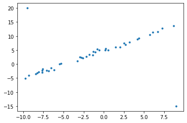
plt.scatter(t,y,marker='.')

<matplotlib.collections.PathCollection at 0x7f5bc8202c88>

Least Square Method

In [4]:

A = np.stack([t,np.ones_like(t)], axis=1)
m,n  = A.shape
# b = np.expand_dims(y,axis=1)
b = y

In [7]:

# Define and solve the CVXPY problem.
x = cp.Variable((n))
cost = cp.sum_squares(A@x - b)
prob = cp.Problem(cp.Minimize(cost))
prob.solve()

# Print result.
print("\nThe optimal value is", prob.value)
print("The optimal x is")
print(x.value)
print("The norm of the residual is ", cp.norm(A@x - b, p=2).value)

The optimal value is 1231.8730454292022
The optimal x is
[0.57548266 4.18406705]
The norm of the residual is  35.09804902596727

In [8]:

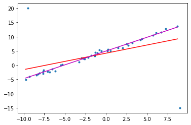
plt.scatter(t,y,marker='.')
i = np.arange(t.min(),t.max(), 0.5)
j = x.value[0]*np.arange(t.min(),t.max(), 0.5) + x.value[1]
plt.plot(i,j,color='r')

[<matplotlib.lines.Line2D at 0x7f5bc00ea518>]

Robust Least Square Method

Least Squard + Huber Penalty Function \({\displaystyle L_{\delta }(a)={\begin{cases}{\frac {1}{2}}{a^{2}}&{\text{for }}|a|\leq \delta ,\\\delta (|a|-{\frac {1}{2}}\delta ),&{\text{otherwise.}}\end{cases}}}\) 위의 panelty 함수는 아래와 같은 형태이다.

Huber loss is green and squared error loss is blue.

이를 cost 함수에 적용하면 에러가 큰 구간에 대해서는 cost가 quadratic에서 linear하게 증가하도록 바뀌어
data point들의 특이점에 대해서 무시하는 효과를 낼 수 있다는 장점이 있다.

In [12]:

x_hub = cp.Variable(n)
hub_cost = cp.sum(cp.huber(A@x_hub - b, M=1))
prob = cp.Problem(cp.Minimize(hub_cost))
prob.solve()

# Print result.
print("\nThe optimal value is", prob.value)
print("The optimal x is")
print(x_hub.value)
print("The norm of the residual is ", cp.norm(cp.huber(A@x_hub - b, M=1), p=1).value)

The optimal value is 113.63173601554703
The optimal x is
[0.96841066 4.9359033 ]
The norm of the residual is  113.63173601554703

In [13]:

plt.scatter(t,y,marker='.')
i = np.arange(t.min(),t.max(), 0.5)
j = x.value[0]*i + x.value[1]
k = x_hub.value[0]*i + x_hub.value[1]
plt.plot(i,j,color='r')
plt.plot(i,k,color='m')

[<matplotlib.lines.Line2D at 0x7f5c013936d8>]

In [None]: