
1
2
3
4
5
6
7
8
9
10
11
12
13
import os, sys, random
import pandas as pd
import matplotlib.pyplot as plt
import numpy as np
from math import sqrt
from sklearn.metrics.pairwise import cosine_similarity
from sklearn.model_selection import train_test_split

sys.path.append("/home/swyoo/algorithm/")
from utils.verbose import logging_time
from ipypb import track, chain

np.set_printoptions(precision=3)
1
2
3
4
5
DFILE = "ml-latest-small"
CHARSET = 'utf8'
ratings = pd.read_csv(os.path.join(DFILE, 'ratings.csv'), encoding=CHARSET)
# tags = pd.read_csv(os.path.join(DFILE, 'tags.csv'), encoding=CHARSET)
movies = pd.read_csv(os.path.join(DFILE, 'movies.csv'), encoding=CHARSET)
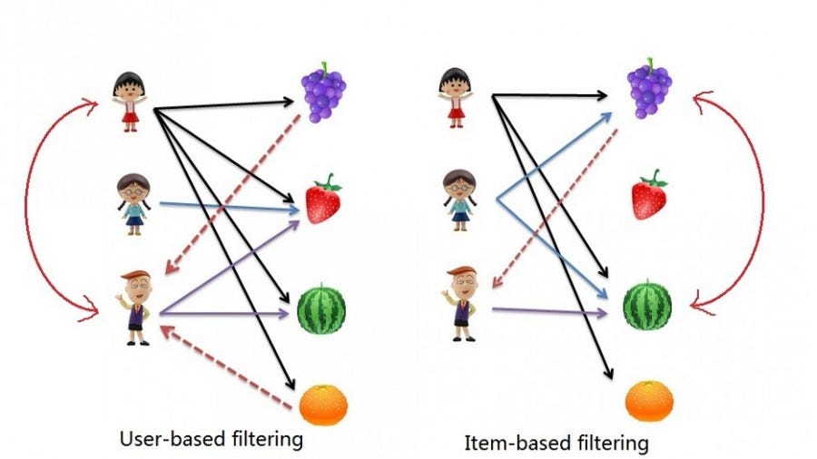
Memory Based Collabortive Filtering
- User-User Collaborative Filtering: Here we find look alike users based on similarity and recommend movies which first user’s look-alike has chosen in past. This algorithm is very effective but takes a lot of time and resources. It requires to compute every user pair information which takes time. Therefore, for big base platforms, this algorithm is hard to implement without a very strong parallelizable system.
- Item-Item Collaborative Filtering: It is quite similar to previous algorithm, but instead of finding user’s look-alike, we try finding movie’s look-alike. Once we have movie’s look-alike matrix, we can easily recommend alike movies to user who have rated any movie from the dataset. This algorithm is far less resource consuming than user-user collaborative filtering. Hence, for a new user, the algorithm takes far lesser time than user-user collaborate as we don’t need all similarity scores between users.
Step 1. Preprocessing
Now I use the scikit-learn library to split the dataset into testing and training. Cross_validation.train_test_split shuffles and splits the data into two datasets according to the percentage of test examples, which in this case is 0.2.
1
2
3
4
5
6
7
8
df_train, df_test = train_test_split(ratings, test_size=0.2, random_state=0, shuffle=True)
df_train.shape, df_test.shape

R = ratings.pivot(index='userId', columns='movieId', values='rating')
M, N = R.shape
print("num_users: {}, num_movies: {}".format(M, N))
print("density rate: {:.2f}%".format((1 - (R.isna().sum(axis=0).sum() / (M * N))) * 100))
R
1
2
3
num_users: 610, num_movies: 9724
density rate: 1.70%
| movieId | 1 | 2 | 3 | 4 | 5 | 6 | 7 | 8 | 9 | 10 | ... | 193565 | 193567 | 193571 | 193573 | 193579 | 193581 | 193583 | 193585 | 193587 | 193609 |
|---|---|---|---|---|---|---|---|---|---|---|---|---|---|---|---|---|---|---|---|---|---|
| userId | |||||||||||||||||||||
| 1 | 4.0 | NaN | 4.0 | NaN | NaN | 4.0 | NaN | NaN | NaN | NaN | ... | NaN | NaN | NaN | NaN | NaN | NaN | NaN | NaN | NaN | NaN |
| 2 | NaN | NaN | NaN | NaN | NaN | NaN | NaN | NaN | NaN | NaN | ... | NaN | NaN | NaN | NaN | NaN | NaN | NaN | NaN | NaN | NaN |
| 3 | NaN | NaN | NaN | NaN | NaN | NaN | NaN | NaN | NaN | NaN | ... | NaN | NaN | NaN | NaN | NaN | NaN | NaN | NaN | NaN | NaN |
| 4 | NaN | NaN | NaN | NaN | NaN | NaN | NaN | NaN | NaN | NaN | ... | NaN | NaN | NaN | NaN | NaN | NaN | NaN | NaN | NaN | NaN |
| 5 | 4.0 | NaN | NaN | NaN | NaN | NaN | NaN | NaN | NaN | NaN | ... | NaN | NaN | NaN | NaN | NaN | NaN | NaN | NaN | NaN | NaN |
| ... | ... | ... | ... | ... | ... | ... | ... | ... | ... | ... | ... | ... | ... | ... | ... | ... | ... | ... | ... | ... | ... |
| 606 | 2.5 | NaN | NaN | NaN | NaN | NaN | 2.5 | NaN | NaN | NaN | ... | NaN | NaN | NaN | NaN | NaN | NaN | NaN | NaN | NaN | NaN |
| 607 | 4.0 | NaN | NaN | NaN | NaN | NaN | NaN | NaN | NaN | NaN | ... | NaN | NaN | NaN | NaN | NaN | NaN | NaN | NaN | NaN | NaN |
| 608 | 2.5 | 2.0 | 2.0 | NaN | NaN | NaN | NaN | NaN | NaN | 4.0 | ... | NaN | NaN | NaN | NaN | NaN | NaN | NaN | NaN | NaN | NaN |
| 609 | 3.0 | NaN | NaN | NaN | NaN | NaN | NaN | NaN | NaN | 4.0 | ... | NaN | NaN | NaN | NaN | NaN | NaN | NaN | NaN | NaN | NaN |
| 610 | 5.0 | NaN | NaN | NaN | NaN | 5.0 | NaN | NaN | NaN | NaN | ... | NaN | NaN | NaN | NaN | NaN | NaN | NaN | NaN | NaN | NaN |
610 rows × 9724 columns
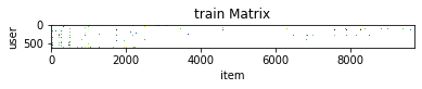
Data sparseness can be visualized as follows.
1
2
3
4
5
6
plt.imshow(R)
plt.grid(False)
plt.xlabel("item")
plt.ylabel("user")
plt.title("train Matrix")
plt.show()
Step 2. Calculate Similarity
At first, calculate similiarity scores for a toy example.
1
2
3
4
5
6
7
8
9
# matrix = [[5,4,None,4,2,None,4,1],[None,5,5,4,2,1,2,None],[1,None,1,5,None,5,3,4]]
# users = ['A','B','C']
# items = ['a','b','c','d','e','f','g','h']

matrix = [[4, None, 5, 5], [4, 2, 1, None], [3, None, 2, 4], [4, 4, None, None], [2, 1, 3, 5]]
users = ['u1', 'u2', 'u3', 'u4', 'u5']
items = ['i1', 'i2', 'i3', 'i4']
df_table = pd.DataFrame(matrix, index=users, columns=items, dtype=float)
df_table
| i1 | i2 | i3 | i4 | |
|---|---|---|---|---|
| u1 | 4.0 | NaN | 5.0 | 5.0 |
| u2 | 4.0 | 2.0 | 1.0 | NaN |
| u3 | 3.0 | NaN | 2.0 | 4.0 |
| u4 | 4.0 | 4.0 | NaN | NaN |
| u5 | 2.0 | 1.0 | 3.0 | 5.0 |
Pearson Similarity
Pearson Similarity can be computed as follows.
Let the number of users be $M$ and the number of items be $N$.
The dimension of pearson correlation similarity matrices for users and items are $ M \times M $, $ N \times N $.
User-Based(UB)
$u, v$ are users
$I$: item set being co-rated by both user $u$ and user $v$
Item-Based(IB)
Note that item-based similarity is modified.
Adjusted cosine similarity is used.
Please see Item-Based Collaborative Filtering Recommendation
Algorithms by Sarwar
\[sim(i, j) = \frac{\sum_{u \in U} (r_{u,i} - \bar{r_u}) (r_{u,j} - \bar{r_u})}{ \sqrt{\sum_{u \in U} (r_{u,i} - \bar{r_u})^2} \sqrt{\sum_{u \in U} (r_{u,j} - \bar{r_u})^2}}\]Basic cosin similarity has one import drawback that difference in rating scale between different users are not takend into account. Therefore, the adjusted cosine similarity offset this drawback by sub-tracking the corresponding user average from each co-rated pair. The formula of adjusted cosine similarity as follows.
$U$: users set that rated both item $i$ and item $j$ (co-rated pair)
1
2
3
4
5
6
7
8
9
10
11
12
13
14
ratings = df_table.to_numpy()
M, N = ratings.shape

def ratedset(ratings, i, kind):
    """ if kind is True, return indices of item set else user set. """
    rates = ratings[i] if kind else ratings[:, i]
    where = np.argwhere(~np.isnan(rates)).flatten()
    return set(where)

def neighbors(ratings, i, j, kind):
    """ return neighbors list. """
    return list(ratedset(ratings, i, kind).intersection(ratedset(ratings, j, kind)))
# neighbors(0, 4, ub=True)
# neighbors(0, 2, ub=False)
1
2
3
4
5
6
7
8
9
10
11
12
13
14
15
16
17
18
19
20
21
22
23
24
25
26
27
28
29
30
31
32
33
34
35
36
37
38
39
40
@logging_time
def pearson(ratings, ub, adjusted=False):
    M, N = ratings.shape
    epsilon = 1e-20
    if ub:
        sim = np.zeros(shape=(M, M), dtype=float)
        for u in track(range(M)):
            for v in range(u, M):
                # find sim(u, v)
                nei = neighbors(ratings, u, v, kind=True) # indices of common items
                if not nei:
                    sim[u][v] = sim[v][u] = np.nan
                    continue
                ru = ratings[u][nei] - np.mean(ratings[u][nei])
                rv = ratings[v][nei] - np.mean(ratings[v][nei])
                up = ru.dot(rv)
                down = sqrt(np.sum(ru**2)) * sqrt(np.sum(rv**2))
                sim[u][v] = sim[v][u] = up / down
        return sim
    else:
        sim = np.zeros(shape=(N, N), dtype=float)
        if adjusted:
            umeans = np.nanmean(ratings, axis=1)
        for i in track(range(N)):
            for j in range(i, N):
                # find sim(i, j)
                nei = neighbors(ratings, i, j, kind=False) # indices of common users
                if not nei:
                    sim[i][j] = sim[j][i] = np.nan
                    continue
                if adjusted:
                    ri = ratings[nei, i] - umeans[nei]
                    rj = ratings[nei, j] - umeans[nei]
                else:
                    ri = ratings[nei, i] - np.mean(ratings[nei, i])
                    rj = ratings[nei, j] - np.mean(ratings[nei, j])
                up = ri.dot(rj)
                down = sqrt(np.sum(ri**2)) * sqrt(np.sum(rj**2))
                sim[i][j] = sim[j][i] = up / down
        return sim
1
df_table
| i1 | i2 | i3 | i4 | |
|---|---|---|---|---|
| u1 | 4.0 | NaN | 5.0 | 5.0 |
| u2 | 4.0 | 2.0 | 1.0 | NaN |
| u3 | 3.0 | NaN | 2.0 | 4.0 |
| u4 | 4.0 | 4.0 | NaN | NaN |
| u5 | 2.0 | 1.0 | 3.0 | 5.0 |
1
2
usim_toy = pearson(ratings, ub=True, verbose=True)
pd.DataFrame(usim_toy, index=users, columns=users)
1
2
/home/swyoo/anaconda3/lib/python3.7/site-packages/ipykernel_launcher.py:18: RuntimeWarning: invalid value encountered in double_scalars
1
2
WorkingTime[pearson]: 5.10669 ms
| u1 | u2 | u3 | u4 | u5 | |
|---|---|---|---|---|---|
| u1 | 1.000000 | -1.000000 | 0.000000 | NaN | 0.755929 |
| u2 | -1.000000 | 1.000000 | 1.000000 | NaN | -0.327327 |
| u3 | 0.000000 | 1.000000 | 1.000000 | NaN | 0.654654 |
| u4 | NaN | NaN | NaN | NaN | NaN |
| u5 | 0.755929 | -0.327327 | 0.654654 | NaN | 1.000000 |
1
2
# pandas library provides calcultation of pearson correlation.
df_table.T.corr(method='pearson', min_periods=1)
| u1 | u2 | u3 | u4 | u5 | |
|---|---|---|---|---|---|
| u1 | 1.000000 | -1.000000 | 0.000000 | NaN | 0.755929 |
| u2 | -1.000000 | 1.000000 | 1.000000 | NaN | -0.327327 |
| u3 | 0.000000 | 1.000000 | 1.000000 | NaN | 0.654654 |
| u4 | NaN | NaN | NaN | NaN | NaN |
| u5 | 0.755929 | -0.327327 | 0.654654 | NaN | 1.000000 |
1
2
3
4
# This calucated values are adjusted cosine similarity
# so, it is different with pearson correlation values.
isim_toy = pearson(ratings, ub=False, adjusted=True, verbose=True)
pd.DataFrame(isim_toy, index=items, columns=items)
1
2
WorkingTime[pearson]: 3.65472 ms
| i1 | i2 | i3 | i4 | |
|---|---|---|---|---|
| i1 | 1.000000 | 0.232485 | -0.787493 | -0.765945 |
| i2 | 0.232485 | 1.000000 | 0.002874 | -1.000000 |
| i3 | -0.787493 | 0.002874 | 1.000000 | -0.121256 |
| i4 | -0.765945 | -1.000000 | -0.121256 | 1.000000 |
1
2
isim_toy_adjust = pearson(ratings, ub=False, adjusted=False, verbose=True)
pd.DataFrame(isim_toy_adjust, index=items, columns=items)
1
2
/home/swyoo/anaconda3/lib/python3.7/site-packages/ipykernel_launcher.py:39: RuntimeWarning: invalid value encountered in double_scalars
1
2
WorkingTime[pearson]: 3.94559 ms
| i1 | i2 | i3 | i4 | |
|---|---|---|---|---|
| i1 | 1.000000 | 0.755929 | 0.050965 | 0.000000 |
| i2 | 0.755929 | 1.000000 | -1.000000 | NaN |
| i3 | 0.050965 | -1.000000 | 1.000000 | 0.755929 |
| i4 | 0.000000 | NaN | 0.755929 | 1.000000 |
1
df_table.corr(method='pearson', min_periods=1)
| i1 | i2 | i3 | i4 | |
|---|---|---|---|---|
| i1 | 1.000000 | 0.755929 | 0.050965 | 0.000000 |
| i2 | 0.755929 | 1.000000 | -1.000000 | NaN |
| i3 | 0.050965 | -1.000000 | 1.000000 | 0.755929 |
| i4 | 0.000000 | NaN | 0.755929 | 1.000000 |
Step 3. Predict unrated scores
User-Based
\(\hat{r}_{a, i} = \bar{r_a} + \frac{ \sum_{b \in nei(i)} sim(a, b) * (r_{b, i} - \bar{r_b})}{\sum_{b \in nei(i)} |sim(a, b)|}\)
where
- $sim(a,b), r_{b, i} - \bar{r_b}$ are scalar.
- $sim(a,b)$ means a pearson similarity score between user a and user b.
- $r_{b, i} - \bar{r_b}$ means a row of normalized rating corresponding to user b.
- $nei(i)$ means users who have rated the item $i$; $\vert nei(i) \vert \le M$
Item-Based
\(\hat{r}_{a, i} = \bar{r_i} + \frac{ \sum_{j \in nei(a)} sim(i, j) * (r_{a, j} - \bar{r_j})}{\sum_{j \in nei(a)} |sim(i, j)|}\) where
- $nei(a)$ means items who “user a” have rated; $\vert nei(a) \vert \le N$
1
2
3
4
5
6
7
8
9
10
11
12
13
14
15
16
17
18
19
20
21
22
23
24
25
26
27
28
29
@logging_time
def predict(ratings, sim, entries, ub):
    epsilon = 1e-20
    sim = np.nan_to_num(sim)

    def pred(a, i):
        if ub:
            nei = list(ratedset(ratings, i, kind=False))  # users set who have rated "movie i".
            if not nei: return np.nanmean(ratings[a])
            ru = np.ones(shape=len(nei))
            for k, u in enumerate(nei):
                overlap = neighbors(ratings, a, u, kind=True)
                ru_mean = np.mean(ratings[u, overlap]) if overlap else 0
                ru[k] = ratings[u][i] - ru_mean
            term = ru.dot(sim[a][nei]) / (epsilon + np.sum(np.abs(sim[a][nei])))
            return np.nanmean(ratings[a]) + term

        else:
            nei = list(ratedset(ratings, a, kind=True)) # items set that "user a" rated.
            if not nei: return np.nanmean(ratings[:, i])
            rj = np.ones(shape=len(nei))
            for k, j in enumerate(nei):
                overlap = neighbors(ratings, i, j, kind=False)
                rj_mean = np.mean(ratings[overlap, j]) if overlap else 0
                rj[k] = ratings[a][j] - rj_mean
            term = rj.dot(sim[i][nei]) / (epsilon + np.sum(np.abs(sim[i][nei])))
            return np.nanmean(ratings[:, i]) + term

    return np.nan_to_num(np.array([pred(u, i) for u, i in track(entries)]))
1
df_table
| i1 | i2 | i3 | i4 | |
|---|---|---|---|---|
| u1 | 4.0 | NaN | 5.0 | 5.0 |
| u2 | 4.0 | 2.0 | 1.0 | NaN |
| u3 | 3.0 | NaN | 2.0 | 4.0 |
| u4 | 4.0 | 4.0 | NaN | NaN |
| u5 | 2.0 | 1.0 | 3.0 | 5.0 |
1
2
3
4
5
6
7
8
9
entries = np.argwhere(np.isnan(ratings))
usim = df_table.T.corr(method='pearson').to_numpy()
isim = df_table.corr(method='pearson').to_numpy()
ub = predict(ratings, usim, entries, ub=True, verbose=True)  # UB
ib = predict(ratings, isim, entries, ub=False, verbose=True)  # IB
print(entries)
print("\npredicted results as follows...")
print(ub)
print(ib)
1
2
WorkingTime[predict]: 12.54416 ms
1
2
3
4
5
6
7
8
9
10
11
WorkingTime[predict]: 7.43055 ms
[[0 1]
 [1 3]
 [2 1]
 [3 2]
 [3 3]]

predicted results as follows...
[3.947 2.341 1.775 4.    4.   ]
[0.912 2.333 2.19  0.408 4.667]
Step 4. Apply to movielen Dataset
1
2
3
4
5
6
7
8
9
10
ratings = pd.read_csv(os.path.join(DFILE, 'ratings.csv'), encoding=CHARSET)

samples = ratings.sample(frac=1)
df_train, df_test = train_test_split(samples, test_size=0.1, random_state=0, shuffle=True)
df_train.shape, df_test.shape

R = samples.pivot(index='userId', columns='movieId', values='rating')
M, N = R.shape
print("num_users: {}, num_movies: {}".format(M, N))
print("density rate: {:.2f}%".format((1 - (R.isna().sum(axis=0).sum() / (M * N))) * 100))
1
2
3
num_users: 610, num_movies: 9724
density rate: 1.70%
1
df_train.shape, df_test.shape
1
((90752, 4), (10084, 4))
1
2
3
4
5
6
mid2idx = {mid: i for i, mid in enumerate(R.columns)}
idx2mid = {v: k for k, v in mid2idx.items()}
uid2idx = {uid: i for i, uid in enumerate(R.index)}
idx2uid = {v: k for k, v in uid2idx.items()}
rmatrix = R.to_numpy().copy()
rmatrix
1
2
3
4
5
6
7
array([[4. , nan, 4. , ..., nan, nan, nan],
       [nan, nan, nan, ..., nan, nan, nan],
       [nan, nan, nan, ..., nan, nan, nan],
       ...,
       [2.5, 2. , 2. , ..., nan, nan, nan],
       [3. , nan, nan, ..., nan, nan, nan],
       [5. , nan, nan, ..., nan, nan, nan]])
4 - 1. conceal test and validation dataset
1
2
3
4
5
6
for uid, mid in zip(df_test.userId, df_test.movieId):
    uidx, midx = uid2idx[uid], mid2idx[mid]
    rmatrix[uidx][midx] = np.nan

rtable = pd.DataFrame(rmatrix, index=uid2idx.keys(), columns=mid2idx.keys())
rtable
| 1 | 2 | 3 | 4 | 5 | 6 | 7 | 8 | 9 | 10 | ... | 193565 | 193567 | 193571 | 193573 | 193579 | 193581 | 193583 | 193585 | 193587 | 193609 | |
|---|---|---|---|---|---|---|---|---|---|---|---|---|---|---|---|---|---|---|---|---|---|
| 1 | 4.0 | NaN | 4.0 | NaN | NaN | 4.0 | NaN | NaN | NaN | NaN | ... | NaN | NaN | NaN | NaN | NaN | NaN | NaN | NaN | NaN | NaN |
| 2 | NaN | NaN | NaN | NaN | NaN | NaN | NaN | NaN | NaN | NaN | ... | NaN | NaN | NaN | NaN | NaN | NaN | NaN | NaN | NaN | NaN |
| 3 | NaN | NaN | NaN | NaN | NaN | NaN | NaN | NaN | NaN | NaN | ... | NaN | NaN | NaN | NaN | NaN | NaN | NaN | NaN | NaN | NaN |
| 4 | NaN | NaN | NaN | NaN | NaN | NaN | NaN | NaN | NaN | NaN | ... | NaN | NaN | NaN | NaN | NaN | NaN | NaN | NaN | NaN | NaN |
| 5 | 4.0 | NaN | NaN | NaN | NaN | NaN | NaN | NaN | NaN | NaN | ... | NaN | NaN | NaN | NaN | NaN | NaN | NaN | NaN | NaN | NaN |
| ... | ... | ... | ... | ... | ... | ... | ... | ... | ... | ... | ... | ... | ... | ... | ... | ... | ... | ... | ... | ... | ... |
| 606 | 2.5 | NaN | NaN | NaN | NaN | NaN | 2.5 | NaN | NaN | NaN | ... | NaN | NaN | NaN | NaN | NaN | NaN | NaN | NaN | NaN | NaN |
| 607 | 4.0 | NaN | NaN | NaN | NaN | NaN | NaN | NaN | NaN | NaN | ... | NaN | NaN | NaN | NaN | NaN | NaN | NaN | NaN | NaN | NaN |
| 608 | 2.5 | 2.0 | 2.0 | NaN | NaN | NaN | NaN | NaN | NaN | 4.0 | ... | NaN | NaN | NaN | NaN | NaN | NaN | NaN | NaN | NaN | NaN |
| 609 | 3.0 | NaN | NaN | NaN | NaN | NaN | NaN | NaN | NaN | NaN | ... | NaN | NaN | NaN | NaN | NaN | NaN | NaN | NaN | NaN | NaN |
| 610 | 5.0 | NaN | NaN | NaN | NaN | 5.0 | NaN | NaN | NaN | NaN | ... | NaN | NaN | NaN | NaN | NaN | NaN | NaN | NaN | NaN | NaN |
610 rows × 9724 columns
1
2
3
M, N = rtable.shape
print("num_users: {}, num_movies: {}".format(M, N))
print("density rate: {:.2f}%".format((1 - (rtable.isna().sum(axis=0).sum() / (M * N))) * 100))
1
2
3
num_users: 610, num_movies: 9724
density rate: 1.53%
4 - 2. calculate similarity and predict ratings.
1
entries = [(uid2idx[uid], mid2idx[mid]) for uid, mid in zip(df_test.userId, df_test.movieId)]
1
2
usim = rtable.T.corr(method='pearson')
upreds = predict(rmatrix, usim, entries, ub=True, verbose=True)
1
2
WorkingTime[predict]: 91141.55078 ms
1
2
isim = rtable.corr(method='pearson')
ipreds = predict(rmatrix, isim, entries, ub=False, verbose=True)
1
2
/home/swyoo/anaconda3/lib/python3.7/site-packages/ipykernel_launcher.py:27: RuntimeWarning: Mean of empty slice
1
2
WorkingTime[predict]: 338750.83947 ms
This calucated values are adjusted cosine similarity
so, it is different with pearson correlation values.
1
isim_adjust = pearson(rmatrix, ub=False, adjusted=True, verbose=True)
1
2
/home/swyoo/anaconda3/lib/python3.7/site-packages/ipykernel_launcher.py:39: RuntimeWarning: invalid value encountered in double_scalars
1
2
WorkingTime[pearson]: 2099248.79313 ms
1
ipreds_adjusted = predict(rmatrix, isim_adjust, entries, ub=False, verbose=True)
1
2
/home/swyoo/anaconda3/lib/python3.7/site-packages/ipykernel_launcher.py:27: RuntimeWarning: Mean of empty slice
1
2
WorkingTime[predict]: 335237.43176 ms
Step 5. Evaluation
There are many evaluation metrics but one of the most popular metric used to evaluate accuracy of predicted ratings is Root Mean Squared Error (RMSE). I will use the mean_square_error (MSE) function from sklearn, where the RMSE is just the square root of MSE.
\[\mathit{RMSE} =\sqrt{\frac{1}{N} \sum (x_i -\hat{x_i})^2}\]1
2
3
4
5
6
7
8
9
10
def rmse(ratings, preds, entries):
""" calculate RMSE
ratings: np.array
preds: List[float]
entries: List[List[int]] """
N = len(preds)
diff = np.zeros_like(preds)
for k, (i, j) in enumerate(entries):
diff[k] = ratings[i][j] - preds[k]
return sqrt(np.sum(diff ** 2) / N)
1
2
3
4
5
6
7
entries = [(uid2idx[uid], mid2idx[mid]) for uid, mid in zip(df_test.userId, df_test.movieId)]
rmse1 = rmse(R.to_numpy(), upreds, entries)
rmse2 = rmse(R.to_numpy(), ipreds, entries)
rmse3 = rmse(R.to_numpy(), ipreds_adjusted, entries)
print('User-based CF RMSE: {:.3f}'.format(rmse1))
print('Item-based CF RMSE: {:.3f}'.format(rmse2))
print('Item-based CF RMSE with ajdusted: {:.3f}'.format(rmse3))
1
2
3
4
User-based CF RMSE: 0.892
Item-based CF RMSE: 1.127
Item-based CF RMSE with ajdusted: 1.151
Recommend Top K Movies
Assume that our recommender system recommends top K movies to a user.
The recommendation precedure is as follows.
- Predict scores for unseen movies by utilizing similarity matrix.
- Sort and determine Top K movies from predicted scores for unseen movies.
- Recommend the top K movies.
Before recommend movies, let’s look at the user’s profile.
1
2
3
4
5
M, N = R.shape
ratings = R.to_numpy()
uid = random.randint(1, M)
print(uid)
R[R.index==uid]
1
2
425
| movieId | 1 | 2 | 3 | 4 | 5 | 6 | 7 | 8 | 9 | 10 | ... | 193565 | 193567 | 193571 | 193573 | 193579 | 193581 | 193583 | 193585 | 193587 | 193609 |
|---|---|---|---|---|---|---|---|---|---|---|---|---|---|---|---|---|---|---|---|---|---|
| userId | |||||||||||||||||||||
| 425 | NaN | 3.0 | NaN | NaN | NaN | 4.0 | NaN | NaN | NaN | 3.0 | ... | NaN | NaN | NaN | NaN | NaN | NaN | NaN | NaN | NaN | NaN |
1 rows × 9724 columns
1
2
3
4
5
seen_indices = np.argwhere(~np.isnan(np.squeeze(R[R.index==uid].to_numpy()))).flatten()
seen = [idx2mid[i] for i in seen_indices]
user_profile = pd.merge(left=movies[movies.movieId.isin(seen)], right=R[R.index==uid][seen].T, on='movieId')
user_profile.columns = ['movieId', 'title', 'genres', 'rating']
user_profile.sort_values(by=['rating'], ascending=False)
| movieId | title | genres | rating | |
|---|---|---|---|---|
| 72 | 778 | Trainspotting (1996) | Comedy|Crime|Drama | 5.0 |
| 37 | 356 | Forrest Gump (1994) | Comedy|Drama|Romance|War | 5.0 |
| 32 | 318 | Shawshank Redemption, The (1994) | Crime|Drama | 5.0 |
| 29 | 293 | Léon: The Professional (a.k.a. The Professiona... | Action|Crime|Drama|Thriller | 5.0 |
| 85 | 1061 | Sleepers (1996) | Thriller | 4.5 |
| ... | ... | ... | ... | ... |
| 259 | 6764 | Rundown, The (2003) | Action|Adventure|Comedy | 2.5 |
| 68 | 736 | Twister (1996) | Action|Adventure|Romance|Thriller | 2.5 |
| 69 | 741 | Ghost in the Shell (Kôkaku kidôtai) (1995) | Animation|Sci-Fi | 2.5 |
| 71 | 762 | Striptease (1996) | Comedy|Crime | 2.5 |
| 64 | 608 | Fargo (1996) | Comedy|Crime|Drama|Thriller | 2.5 |
306 rows × 4 columns
1
2
3
4
5
6
7
8
9
def recommend(R, sim, uid, K):
    """ R: pandas.Dataframe, rating pivot. """
    rates = np.squeeze(R[R.index==uid].to_numpy())
    empties = np.argwhere(np.isnan(rates)).flatten()
    entries = [(uid, mid) for mid in empties]
    preds = predict(ratings, sim, entries, ub=True, verbose=True)
    topK_indices = np.argsort(preds)[-K:][::-1]
    topK = [idx2mid[idx] for idx in topK_indices]
    return topK
1
2
3
topK = recommend(R, usim, uid, K=10)
print(topK)
movies[movies.movieId.isin(topK)]
1
2
3
WorkingTime[predict]: 13215.18350 ms
[6863, 63768, 87867, 60941, 147250, 72603, 5959, 7264, 7394, 5328]
| movieId | title | genres | |
|---|---|---|---|
| 3807 | 5328 | Rain (2001) | Drama|Romance |
| 4143 | 5959 | Narc (2002) | Crime|Drama|Thriller |
| 4608 | 6863 | School of Rock (2003) | Comedy|Musical |
| 4861 | 7264 | An Amazing Couple (2002) | Comedy|Romance |
| 4929 | 7394 | Those Magnificent Men in Their Flying Machines... | Action|Adventure|Comedy |
| 6812 | 60941 | Midnight Meat Train, The (2008) | Horror|Mystery|Thriller |
| 6899 | 63768 | Tattooed Life (Irezumi ichidai) (1965) | Crime|Drama |
| 7195 | 72603 | Merry Madagascar (2009) | Animation |
| 7637 | 87867 | Zookeeper (2011) | Comedy |
| 9138 | 147250 | The Adventures of Sherlock Holmes and Doctor W... | (no genres listed) |
1
2
3
topK = recommend(R, isim, uid, K=10)
print(topK)
movies[movies.movieId.isin(topK)]
1
2
3
WorkingTime[predict]: 14716.72630 ms
[166558, 4215, 4235, 4234, 4233, 4232, 4231, 4229, 4228, 4226]
| movieId | title | genres | |
|---|---|---|---|
| 3132 | 4215 | Revenge of the Nerds II: Nerds in Paradise (1987) | Comedy |
| 3141 | 4226 | Memento (2000) | Mystery|Thriller |
| 3142 | 4228 | Heartbreakers (2001) | Comedy|Crime|Romance |
| 3143 | 4229 | Say It Isn't So (2001) | Comedy|Romance |
| 3144 | 4231 | Someone Like You (2001) | Comedy|Romance |
| 3145 | 4232 | Spy Kids (2001) | Action|Adventure|Children|Comedy |
| 3146 | 4233 | Tomcats (2001) | Comedy |
| 3147 | 4234 | Tailor of Panama, The (2001) | Drama|Thriller |
| 3148 | 4235 | Amores Perros (Love's a Bitch) (2000) | Drama|Thriller |
| 9435 | 166558 | Underworld: Blood Wars (2016) | Action|Horror |
1
2
3
topK = recommend(R, isim_adjust, uid, K=10)
print(topK)
movies[movies.movieId.isin(topK)]
1
2
3
WorkingTime[predict]: 15062.08897 ms
[70301, 72696, 6577, 1024, 3689, 6301, 4883, 1551, 1490, 81156]
| movieId | title | genres | |
|---|---|---|---|
| 782 | 1024 | Three Caballeros, The (1945) | Animation|Children|Musical |
| 1139 | 1490 | B*A*P*S (1997) | Comedy |
| 1170 | 1551 | Buddy (1997) | Adventure|Children|Drama |
| 2751 | 3689 | Porky's II: The Next Day (1983) | Comedy |
| 3566 | 4883 | Town is Quiet, The (Ville est tranquille, La) ... | Drama |
| 4313 | 6301 | Straw Dogs (1971) | Drama|Thriller |
| 4454 | 6577 | Kickboxer 2: The Road Back (1991) | Action|Drama |
| 7092 | 70301 | Obsessed (2009) | Crime|Drama|Thriller |
| 7201 | 72696 | Old Dogs (2009) | Comedy |
| 7442 | 81156 | Jackass 3D (2010) | Action|Comedy|Documentary |
Reference
[1] Item-Based Recommender System original paper written by sarwar 2001
[2] Survey paper
[3] Korean Blog
[4] English Blog

Leave a comment