Pandas simple tutorial

In [1]:

import pymysql, argparse, os, sys, json
from sqlalchemy import create_engine
import pandas as pd
import matplotlib.pyplot as plt

In [2]:

parser = argparse.ArgumentParser()
parser.add_argument('-user', help="mysql database user", type=str, required=False, default='****')
parser.add_argument('-pw', help="password", type=str, required=False, default='****')
parser.add_argument('-host', help="ip address", type=str, required=False, default='***.***.***.***')
parser.add_argument('-db', help="database name", type=str, required=False, default='classicmodels')
parser.add_argument('-charset', help="character set to use", type=str, required=False, default='utf8mb4')
sys.argv = ['-f']
args = parser.parse_args()
print(args)
con = pymysql.connect(host=args.host, user=args.user, password=args.pw, use_unicode=True, charset=args.charset)
cursor = con.cursor()

Namespace(charset='utf8mb4', db='classicmodels', host='***.***.***.***', pw='****', user='****')

In [3]:

# helper functions 
sql = lambda command: pd.read_sql(command, con)
def fetch(command):
    cursor.execute(command)
    return cursor.fetchall()

# db_data = 'mysql+pymysql://' + '<USER-NAME>' + ':' + '<PASSWORD>' + '@' + '***.***.***.***' + ':3306/' + '<DB-NAME>' + '?charset=utf8mb4'
db_data = "mysql+pymysql://{}:{}@{}:3306/{}?charset={}".format(args.user, args.pw, args.host, args.db, args.charset)
engine = create_engine(db_data).connect()

fetch("use classicmodels")

()

Pandas Tutorial

Prerequisite

1. How to use pymysql and mysql
2. How to use argparse module in jupyter notebook

I use sample database classicmodels on MySQL in this tutorial

In [4]:

sql("show tables")

	Tables_in_classicmodels
0	customers
1	employees
2	music
3	offices
4	orderdetails
5	orders
6	payments
7	productlines
8	products

In [5]:

df = sql("select * from customers")

In [6]:

df.info()

<class 'pandas.core.frame.DataFrame'>
RangeIndex: 122 entries, 0 to 121
Data columns (total 13 columns):
 #   Column                  Non-Null Count  Dtype  
---  ------                  --------------  -----  
 0   customerNumber          122 non-null    int64  
 1   customerName            122 non-null    object 
 2   contactLastName         122 non-null    object 
 3   contactFirstName        122 non-null    object 
 4   phone                   122 non-null    object 
 5   addressLine1            122 non-null    object 
 6   addressLine2            22 non-null     object 
 7   city                    122 non-null    object 
 8   state                   49 non-null     object 
 9   postalCode              115 non-null    object 
 10  country                 122 non-null    object 
 11  salesRepEmployeeNumber  100 non-null    float64
 12  creditLimit             122 non-null    float64
dtypes: float64(2), int64(1), object(10)
memory usage: 12.5+ KB

Indexing and selecting

In [7]:

df.head(n=1)

	customerNumber	customerName	contactLastName	contactFirstName	phone	addressLine1	addressLine2	city	state	postalCode	country	salesRepEmployeeNumber	creditLimit
0	103	Atelier graphique	Schmitt	Carine	40.32.2555	54, rue Royale	None	Nantes	None	44000	France	1370.0	21000.0

In [8]:

df.iloc[0]

customerNumber                          103
customerName              Atelier graphique
contactLastName                     Schmitt
contactFirstName                    Carine 
phone                            40.32.2555
addressLine1                 54, rue Royale
addressLine2                           None
city                                 Nantes
state                                  None
postalCode                            44000
country                              France
salesRepEmployeeNumber                 1370
creditLimit                           21000
Name: 0, dtype: object

In [9]:

df.sort_values(by='creditLimit')[:3]

	customerNumber	customerName	contactLastName	contactFirstName	phone	addressLine1	addressLine2	city	state	postalCode	country	salesRepEmployeeNumber	creditLimit
74	335	Cramer Spezialitäten, Ltd	Cramer	Philip	0555-09555	Maubelstr. 90	None	Brandenburg	None	14776	Germany	NaN	0.0
41	223	Natürlich Autos	Kloss	Horst	0372-555188	Taucherstraße 10	None	Cunewalde	None	01307	Germany	NaN	0.0
44	237	ANG Resellers	Camino	Alejandra	(91) 745 6555	Gran Vía, 1	None	Madrid	None	28001	Spain	NaN	0.0

In [10]:

df.sort_values(by='creditLimit')[['customerNumber', 'phone', 'city', 'creditLimit']]

	customerNumber	phone	city	creditLimit
74	335	0555-09555	Brandenburg	0.0
41	223	0372-555188	Cunewalde	0.0
44	237	(91) 745 6555	Madrid	0.0
48	247	069-0555984	Frankfurt	0.0
109	465	+34 913 728555	Madrid	0.0
...	...	...	...	...
29	187	(171) 555-1555	Manchester	136800.0
15	151	2125557413	NYC	138500.0
60	298	0897-034555	Genève	141300.0
5	124	4155551450	San Rafael	210500.0
10	141	(91) 555 94 44	Madrid	227600.0

122 rows × 4 columns

Merge and Join

In [11]:

df2 = sql("select * from orders")

In [12]:

df2.head(n=2)

	orderNumber	orderDate	requiredDate	shippedDate	status	comments	customerNumber
0	10100	2003-01-06	2003-01-13	2003-01-10	Shipped	None	363
1	10101	2003-01-09	2003-01-18	2003-01-11	Shipped	Check on availability.	128

In [13]:

len(pd.merge(left=df, right=df2))

326

In [14]:

# sanity check through sql.
sql("select count(*) from customers c, orders o where c.customerNumber = o.customerNumber")

	count(*)
0	326

Pivot table

In [15]:

df = sql("select * from music")
df.head(n=2)
df = df.pivot(index='user_id', columns='item_id', values='ratings')
num_user, num_items = df.shape
print("# of users: {:,}, # of items: {:,}".format(num_user, num_items))
df.head(n=3)

# of users: 1,429, # of items: 900

item_id	0	1	2	3	4	5	6	7	8	9	...	890	891	892	893	894	895	896	897	898	899
user_id
0	NaN	NaN	NaN	NaN	NaN	NaN	NaN	NaN	NaN	NaN	...	NaN	NaN	NaN	NaN	NaN	NaN	NaN	NaN	NaN	NaN
1	NaN	NaN	NaN	NaN	NaN	NaN	NaN	NaN	NaN	NaN	...	NaN	NaN	NaN	NaN	NaN	NaN	NaN	NaN	NaN	NaN
2	NaN	NaN	NaN	NaN	NaN	NaN	NaN	NaN	NaN	NaN	...	NaN	NaN	NaN	NaN	NaN	NaN	NaN	NaN	NaN	NaN

3 rows × 900 columns

In [16]:

"density rate: {:.3f}%".format((1 - (df.isna().sum(axis=0).sum() / (num_user * num_items))) * 100)

'density rate: 0.798%'

Visualization

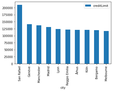
I would like to know order statistics for people with a large credit limit group by city of residence in the customer table.

In [17]:

df = sql("select * from customers")

In [18]:

df.head(n=1)

	customerNumber	customerName	contactLastName	contactFirstName	phone	addressLine1	addressLine2	city	state	postalCode	country	salesRepEmployeeNumber	creditLimit
0	103	Atelier graphique	Schmitt	Carine	40.32.2555	54, rue Royale	None	Nantes	None	44000	France	1370.0	21000.0

In [19]:

sql("select count(distinct city) from customers where creditLimit > 1000")

	count(distinct city)
0	77

In [20]:

res = sql(
    """ select city, avg(creditLimit) as creditLimit
        from customers 
        where creditLimit > 0 
        group by city 
        order by creditLimit""")

In [21]:

res.head(n=3)

	city	creditLimit
0	Charleroi	23500.0
1	Glendale	30350.0
2	Milan	34800.0

To simplify this problem, let’s pick top 10 countries.

In [22]:

res = res.nlargest(n=10, columns='creditLimit')

In [23]:

plt.figure()
res.plot(x='city', y='creditLimit', kind='bar')

<matplotlib.axes._subplots.AxesSubplot at 0x7f03a54a8810>

<Figure size 432x288 with 0 Axes>

---

ETC

Apply function to row-wise(axis=1) or column-wise(axis=0)

In [24]:

def func(x):
    import pdb; pdb.set_trace()
    return  x
df.apply(lambda x: x['city'], axis=1)

0            Nantes
1         Las Vegas
2         Melbourne
3            Nantes
4           Stavern
           ...     
117    Philadelphia
118        Brisbane
119          London
120          Boston
121      Auckland  
Length: 122, dtype: object

Export pandas.DataFrame to csv file.

In [25]:

df.to_csv('./customers.csv')

Options

Display options

In [26]:

# display options 
pd.set_option('display.max_columns', None)
pd.set_option('display.max_rows', None)
pd.set_option('display.max_colwidth', None)
# pd.reset_option('^display') # reset options of starting with 'display'.

Referenece

[1]Offical pandas Guide
[2]MySQL sample database description