
1
2
3
4
5
6
7
8
9
10
11
12
import random
import logging
from typing import Dict, List, Tuple

import numpy as np
import pandas as pd
import matplotlib.pyplot as plt
from scipy.stats import multivariate_normal as mvn
from sklearn.metrics import confusion_matrix
from sklearn.metrics import precision_score
from sklearn.metrics import recall_score
from sklearn.model_selection import train_test_split
1
2
import platform
print(platform.python_version())
1
2
3.8.3
EM algorithm for GMM
Let’s study about EM(expectation-maximization) algorithm for GMM(gaussian mixture model) wikipedia.
Unsupervised problem can be solved by EM-algorithm.
If you want to know about kmeans or kmedoid model in EM-algorithm category, please look at this posting.
In this time, we will apply EM algorithm, especially GMM to a solve clustering problem.
A toy example is as follows.
1
2
3
4
5
6
7
8
9
10
11
12
13
14
# Load data
toy = np.load('./data/clustering/data_4_1.npy') # data_1, for visualization
dataset = np.load('./data/clustering/data_4_2.npz') # data_2, for test
X = dataset['X']
y = dataset['y']

# Sanity check
print('data shape: ', toy.shape) # (1500, 2)
print('X shape: ', X.shape) # (1500, 6)
print('y shape: ', y.shape) # (1500,)

df_toy = pd.DataFrame(toy, columns=['f1', 'f2'])
df_toy.head()  # toy example does not have ground truth label.
toy_range = list(zip(df_toy.min(), df_toy.max()))
1
2
3
4
data shape:  (1500, 2)
X shape:  (1500, 6)
y shape:  (1500,)
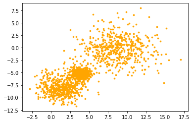
\(\require{color}\) visualize toy example.
1
2
toy = df_toy.to_numpy()
plt.scatter(toy[:,0], toy[:,-1], color='orange', s=7)
1
<matplotlib.collections.PathCollection at 0x7f51f9643910>
1
2
3
4
5
features = ['f1', 'f2', 'f3', 'f4', 'f5', 'f6']
dataset = pd.DataFrame(X, columns=features)
dataset = pd.merge(left=dataset, right=pd.DataFrame(y, columns=['label']), on=dataset.index)
dataset = dataset[features + ['label']]
dataset.head()
| f1 | f2 | f3 | f4 | f5 | f6 | label | |
|---|---|---|---|---|---|---|---|
| 0 | 4.200999 | -0.506804 | -0.024489 | -0.039783 | 0.067635 | -0.029724 | 2 |
| 1 | 4.572715 | 1.414097 | 0.097670 | 0.155350 | -0.058382 | 0.113278 | 0 |
| 2 | 9.183954 | -0.163354 | 0.045867 | -0.257671 | -0.015087 | -0.047957 | 1 |
| 3 | 8.540300 | 0.308409 | 0.007325 | -0.068467 | -0.130611 | -0.016363 | 2 |
| 4 | 8.995599 | 1.275279 | -0.015923 | 0.062932 | -0.072392 | 0.034399 | 0 |
1
2
3
# exploration
print("min info:\n", dataset.min())
print("max info:\n", dataset.max())
1
2
3
4
5
6
7
8
9
10
11
12
13
14
15
16
17
18
19
min info:
 f1       -2.802532
f2      -11.719322
f3       -0.291218
f4       -0.378744
f5       -0.336366
f6       -0.383337
label     0.000000
dtype: float64
max info:
 f1       17.022084
f2        7.953588
f3        0.402071
f4        0.310862
f5        0.316762
f6        0.342837
label     2.000000
dtype: float64
EM Algorithm
Given dataset $X$,
EM-algorithm aims to find parameter values that maximize liklihood $P(X \vert \theta)$.
Generally, the EM-algorithm has 2 steps.
Expectation
Find expectation of the (log) liklihood $log P(X \vert \theta)$ on the conditional distribution of $Z \vert X, \theta^t$,
where $Z$ is latent variable(e.g., clustered labels) and $\theta$ is model parameters(e.g., $\mu, \Sigma$).
The key concept is marginalizing liklihood $P(X \vert \theta)$ for $Z$. \(\require{cancel}\) \(\begin{align} P(X \vert \theta) = \sum_{Z} P(X, Z \vert \theta) = \sum_{Z} P(X \vert Z, \theta) P(Z \vert \theta) \end{align}\)
Therefore, \(\begin{align} Q(\theta \vert \theta^t) &= \mathbb{E}_{Z| X, \theta^t} [log P(X \vert \theta)] = \sum_{Z} P(Z| X, \theta^t) log \left( P(X \vert Z, \theta) P(Z \vert \theta) \right) \end{align}\)
Maximization
Find $\theta^{t + 1}$ maximizing $Q$. \(\theta^{t + 1} = \underset{\theta}{argmax} Q(\theta \vert \theta^t)\)
GMM
GMM is a special case of EM algorithm.
We will solve a clustering problem, so let $Z$ be random varible, which means a class label.
At this time, please notice as follows for simplifying notations. \(\begin{align} z_k \triangleq \mathcal{I} (Z = k) \\ \end{align}\)
Gaussian Mixture Model is iterally ensemble of multiple normal distribution as follows. [src: https://en.wikipedia.org/wiki/File:Movie.gif]

For GMM, assume that $z_k \sim \mathcal{N}(\mu_k, \Sigma_k), \forall k$, where $k$ is an index of a class.
Also, model parameter $\theta = {\mu_k, \Sigma_k, \pi_k }_{k=1, \cdots, K}$, where K is the number of classes.
GMM: Expectation
For GMM, expectation of the (log) liklihood on the conditional distribution of $Z$ as follows.
The following formula is calculated considering all datasets and all classes. \(\begin{align} Q(\theta \vert \theta^t) &= \sum_n \sum_k \textcolor{red}{P(z_k| x_n, \theta^t)} log \left( P(x_n \vert z_k, \theta) P(z_k \vert \theta) \right) \\ \textcolor{red}{P(z_k| x_n, \theta^t)} &= \frac{P(x_n, \theta^t, z_k)}{P(x_n, \theta^t)} &\text{bayes' rule} \\ &= \frac{P(x_n, \theta^t \vert z_k) P(z_k)}{\sum_{k} P(x_n, \theta^t \vert z_k) P(z_k)} \\ &= \frac{\textcolor{pink}{P(x_n; \mu_k^t, \Sigma_{k}^t)} \pi_k^t}{\sum_{k} \textcolor{pink}{P(x_n; \mu_k^t, \Sigma_{k}^t)} \pi_k^t} &\text{prob chain rule and where }\pi_k = P(z_k) \text{ s.t } \sum_k \pi_k = 1 \\ \textcolor{pink}{P(x_n; \mu_k^t, \Sigma_{k}^t)} &= \frac{1}{\sqrt { (2\pi)^d \vert \Sigma_k^t \vert } } \exp\left(-\frac{1}{2} (x_n - \mu_k^t )^{\rm T} (\Sigma_{k}^{t})^{-1} ({x_n}-\mu_k^t)\right)\\ P(x_n \vert z_k, \theta) &= \frac{1}{\sqrt { (2\pi)^d \vert \Sigma_k \vert } } \exp\left(-\frac{1}{2} (x_n - \mu_k )^{\rm T} \Sigma_{k}^{-1} ({x_n}-\mu_k)\right) \\ P(z_k \vert \theta) &= \pi_k \\ log \left( P(x_n \vert z_k, \theta) P(z_k \vert \theta) \right) &= -\frac{1}{2} \left( d \log(2\pi) + \log(\vert \Sigma_k \vert) + (x_n - \mu_k )^{\rm T} \Sigma_{k}^{-1} ({x_n}-\mu_k) \right) + log \pi_k \end{align}\)
To simplify notation, $\textcolor{red}{\gamma^t(z_{nk})}$ is defined as follows. \(\begin{align} \gamma^t(z_{nk}) &\triangleq \frac{P(x_n; \mu_k^t, \Sigma_{k}^t) \pi_k^t}{\sum_{k} p(x_n; \mu_k^t, \Sigma_{k}^t) \pi_k^t} \end{align}\)
$\gamma^t(z_{nk})$ is the key in this step (because only this value is used at m-step updating rule).
Please notice that $log P(x_n \vert z_k, \theta)$ term does not used in maximization step later.
Therefore, store only $\gamma^t(z_{nk}) \in \mathbb{R}, \forall n, k$.
$\gamma^t(z_{nk})$ means a normalized weight component for $z_{nk} \sim \mathcal{N}(\mu^t_k, \Sigma^t_k)$.
GMM: Maximization
recall that \(\theta^{t + 1} = \underset{\theta}{argmax} Q(\theta \vert \theta^t)\)
For GMM, $Q(\theta \vert \theta^t)$ is divided into two parts (warnnig: $\pi_k$ is prior, but $\pi = 3.14$). \(\begin{align} Q(\theta \vert \theta^t) &= \sum_n \sum_k \gamma^t(z_{nk}) \left( -\frac{1}{2} \left( d \log(2\pi) + \log(\vert \Sigma_k \vert) + (x_n - \mu_k )^{\rm T} \Sigma_{k}^{-1} ({x_n}-\mu_k) \right) + log \pi_k \right)\\ &= \sum_n \sum_k \textcolor{red}{\gamma^t(z_{nk}) (-\frac{d}{2} \log(2\pi) + log \pi_k)} + -\frac{1}{2} \textcolor{pink}{\gamma^t(z_{nk}) \left( \log(\vert \Sigma_k \vert) + (x_n - \mu_k )^{\rm T} \Sigma_{k}^{-1} ({x_n}-\mu_k) \right)} \end{align}\)
From the first part, $\pi_k^{t+1}$ is determined as follows. \(\pi_k^{t + 1} = \underset{\pi}{argmax} \sum_{n}\sum_{k} \gamma^t(z_{nk}) log\pi_k \text{ subject to }\sum_k \pi_k = 1\)
Using lagrangian method, get a cost function. and then, apply partial derivative for the first part($\frac{\partial}{\partial \pi_k^t}$) updating formula can be found as follows. \(\begin{align} \pi_k^{t + 1} &= \frac{\sum_n \gamma^t(z_{nk})}{\sum_k \sum_n \gamma^t(z_{nk})} \\ &= \frac{\sum_n \gamma^t(z_{nk})}{\sum_n 1} & \text{since } \sum_k \gamma_r(z_{nk}) = 1 \\ &= \frac{1}{N}\sum_n \gamma^t(z_{nk}) \end{align}\)
From the second part, $\mu_k^{t+1}, \Sigma_k^{t + 1}$ is determined as follows. \((\mu_k^{t + 1}, \Sigma_k^{t + 1}) = \underset{(\mu_k, \Sigma_k)}{argmin} \sum_{n}\sum_{k} \gamma^t(z_{nk}) \left( \log(\vert \Sigma_k \vert) + (x_n - \mu_k )^{\rm T} \Sigma_{k}^{-1} ({x_n}-\mu_k) \right)\)
Partial derivative for second part($\frac{\partial}{\partial \mu_k^t}, \frac{\partial}{\partial \Sigma_k^t}$) deduce updating formula as follows.
\[\begin{align} \mu_k^{t + 1} &= \frac{\sum_n \gamma^t(z_{nk}) x_n}{\sum_n \gamma^t(z_{nk})} \\ \Sigma_k^{t + 1} &= \frac{\sum_n \gamma^t(z_{nk}) (x_n - \mu_k^{t+ 1})(x_n - \mu_k^{t+ 1})^{\rm T}}{\sum_n \gamma^t(z_{nk})} \end{align}\]This is pseudo code.

After $T$ step, the GMM model returns $K$ gaussian distributions.
1
2
3
4
5
6
7
8
9
10
11
12
13
14
15
16
17
18
19
20
21
22
23
24
25
26
27
28
29
30
31
32
33
34
35
36
37
38
39
40
41
42
43
44
45
46
47
48
49
50
51
52
53
54
55
56
57
58
59
60
61
62
63
64
65
66
67
68
69
70
71
72
73
74
75
76
77
78
79
80
81
82
83
84
85
86
87
88
89
90
91
92
93
94
95
96
97
98
99
100
101
102
103
104
105
106
107
108
109
110
111
112
113
114
115
class GMM:
    def __init__(self, K: int, log_mode='file'):
        self.K = K
        self.logger = logging.getLogger("GMM")
        self.set_logging_format(log_mode)

    def set_logging_format(self, log_mode):
        self.logger.setLevel(logging.DEBUG)
        if log_mode == 'file':
            handler = logging.FileHandler('GMM.log')
        else:
            handler = logging.StreamHandler()
        handler.setLevel(logging.DEBUG)
        handler.setFormatter(logging.Formatter("%(asctime)s - %(name)s - %(levelname)s - %(message)s"))
        self.logger.addHandler(handler)

    def initialize(self, X: np.array, X_range=None):
        self.N, self.D = X.shape
        self.pi = np.ones(shape=(self.K)) / self.K
        if X_range:
            self.mu = np.zeros((self.K, self.D))
            for k in range(self.K):
                for d, (min_v, max_v) in enumerate(X_range):
                    self.mu[k][d] = np.random.uniform(low=min_v, high=max_v)
        else:
            self.mu = np.tile(np.mean(X, axis=0),(self.K, 1))
            self.mu += np.random.normal(loc=0,scale=1,size=self.mu.shape)

        self.sigma = np.tile(np.eye(self.D),(self.K, 1, 1))
        self.gamma = None


    def _e_step(self, X, pi, mu, sigma):
        """Performs E-step on GMM model

        Parameters:
        ------------
        X: (N x D), data points
        pi: (K), weights of mixture components
        mu: (K x D), mixture component means
        sigma: (K x D x D), mixture component covariance matrices

        Returns:
        ----------
        gamma: (N x K), probabilities of clusters for objects
        """
        assert (self.N, self.D) == X.shape, "ERROR: X.shape is not valid"
        self.gamma = np.zeros((self.N, self.K))

        for k in range(self.K):
            # Posterior Distribution using Bayes Rule
            self.gamma[:,k] = self.pi[k] * mvn.pdf(X, self.mu[k,:], self.sigma[k]) # N x 1

        # normalize across columns to make a valid probability
        gamma_norm = np.sum(self.gamma, axis=1)[:,np.newaxis]
        self.gamma /= gamma_norm

        return self.gamma

    def _m_step(self, X, gamma):
        """Performs M-step of the GMM
        We need to update our priors, our means
        and our covariance matrix.

        Parameters:
        -----------
        X: (N x D), data
        gamma: (N x K), posterior distribution of lower bound

        Returns:
        ---------
        pi: (K)
        mu: (K x D)
        sigma: (K x D x D)
        """
        # responsibilities for each gaussian
        self.pi = np.mean(self.gamma, axis = 0)
        self.mu = np.dot(self.gamma.T, X) / np.sum(self.gamma, axis = 0)[:,np.newaxis]

        for k in range(self.K):
            x = X - self.mu[k, :] # (N x d)

            gamma_diag = np.diag(self.gamma[:,k])
            x_mu = np.matrix(x)
            gamma_diag = np.matrix(gamma_diag)

            sigma_k = x.T * gamma_diag * x
            self.sigma[k,:,:]=(sigma_k) / np.sum(self.gamma[:,k], axis=0, keepdims=True)[:,np.newaxis]

        return self.pi, self.mu, self.sigma

    def fit(self, X, X_range=None, iters=5):
        """Compute the E-step and M-step and
            Calculates the lowerbound

        Parameters:
        -----------
        X: (N x d), data

        Returns:
        ----------
        instance of GMM
        """
        self.initialize(X, X_range)

        for run in range(iters):
            self.gamma  = self._e_step(X, self.mu, self.pi, self.sigma)
            self.pi, self.mu, self.sigma = self._m_step(X, self.gamma)
            self.logger.info("PI: {}, MU: {}".format(self.pi, self.mu))

    def predict(self, X):
        predictions = np.zeros((X.shape[0], self.K))
        for k in range(self.K):
            predictions[:,k] = self.pi[k] * mvn.pdf(X, self.mu[k,:], self.sigma[k])
        return np.argmax(predictions, axis=1)
1
2
3
4
data = toy
data_range = toy_range
model = GMM(K=2, log_mode='file')
model.fit(data, data_range, iters=0)
1
2
3
print("means:\n", model.mu)
print()
print("sigma:\n", model.sigma)
1
2
3
4
5
6
7
8
9
10
11
means:
 [[ 5.52318009 -4.35115003]
 [16.78627291  0.39553948]]

sigma:
 [[[1. 0.]
  [0. 1.]]

 [[1. 0.]
  [0. 1.]]]
Prediction is conducted by $\gamma(z^*_{nk})$ as follows.

1
2
predictions = model.predict(data)
predictions
1
array([1, 0, 0, ..., 0, 0, 0])
Visualization
1
2
3
4
5
6
7
8
9
10
11
12
13
14
15
16
17
18
19
# Credit to python data science handbook for the code to plot these distributions
from matplotlib.patches import Ellipse

def draw_ellipse(position, covariance, ax=None, **kwargs):
    """Draw an ellipse with a given position and covariance"""
    ax = ax or plt.gca()

    # Convert covariance to principal axes
    if covariance.shape == (2, 2):
        U, s, Vt = np.linalg.svd(covariance)
        angle = np.degrees(np.arctan2(U[1, 0], U[0, 0]))
        width, height = 2 * np.sqrt(s)
    else:
        angle = 0
        width, height = 2 * np.sqrt(covariance)

    # Draw the Ellipse
    for nsig in range(1, 4):
        ax.add_patch(Ellipse(position, nsig * width, nsig * height, angle, **kwargs))
1
2
3
4
5
6
7
8
9
10
11
12
13
14
15
16
17
18
19
20
21
22
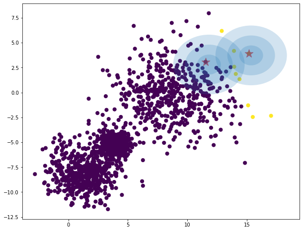
data = toy
data_range = toy_range
iterations = 0
model = GMM(K=2, log_mode='file')
model.fit(data, data_range, iters=iterations)
predictions = model.predict(data)
# compute centers as point of highest density of distribution
# the mode is mean for gaussian distribution.
K = 2
centers = np.zeros((K, data.shape[1])) # red points
for i in range(K):
density = mvn(cov=model.sigma[i], mean=model.mu[i]).logpdf(data)
centers[i, :] = data[np.argmax(density)]
plt.figure(figsize = (10,8))
plt.scatter(data[:, 0], data[:, 1], c=predictions, s=50, cmap='viridis')
plt.scatter(centers[:, 0], centers[:, 1], c='red', marker='*', s=300, alpha=0.6);
w_factor = 0.2 / model.pi.max()
for pos, covar, w in zip(model.mu, model.sigma, model.pi):
draw_ellipse(pos, covar, alpha=w * w_factor)
1
2
3
4
5
6
7
8
9
10
11
12
13
14
15
16
17
18
19
20
21
22
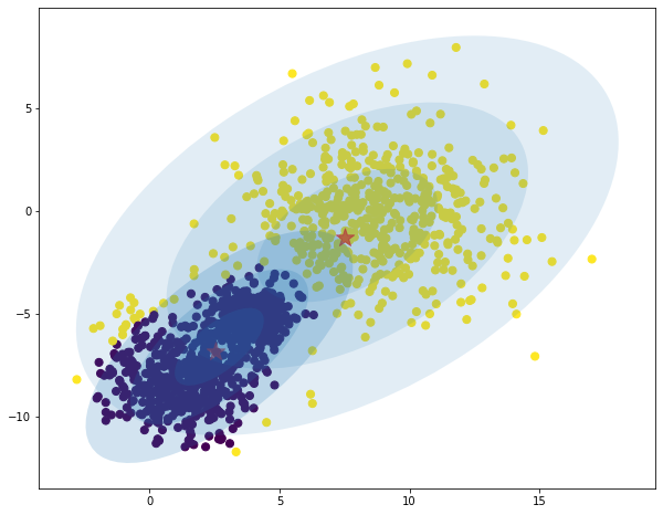
data = toy
data_range = toy_range
iterations = 20
model = GMM(K=2, log_mode='file')
model.fit(data, data_range, iters=iterations)
predictions = model.predict(data)
# compute centers as point of highest density of distribution
# the mode is mean for gaussian distribution.
K = 2
centers = np.zeros((K, data.shape[1])) # red points
for i in range(K):
density = mvn(cov=model.sigma[i], mean=model.mu[i]).logpdf(data)
centers[i, :] = data[np.argmax(density)]
plt.figure(figsize = (10,8))
plt.scatter(data[:, 0], data[:, 1], c=predictions, s=50, cmap='viridis')
plt.scatter(centers[:, 0], centers[:, 1], c='red', marker='*', s=300, alpha=0.6);
w_factor = 0.2 / model.pi.max()
for pos, covar, w in zip(model.mu, model.sigma, model.pi):
draw_ellipse(pos, covar, alpha=w * w_factor)
Test
1
dataset.head()
| f1 | f2 | f3 | f4 | f5 | f6 | label | |
|---|---|---|---|---|---|---|---|
| 0 | 4.200999 | -0.506804 | -0.024489 | -0.039783 | 0.067635 | -0.029724 | 2 |
| 1 | 4.572715 | 1.414097 | 0.097670 | 0.155350 | -0.058382 | 0.113278 | 0 |
| 2 | 9.183954 | -0.163354 | 0.045867 | -0.257671 | -0.015087 | -0.047957 | 1 |
| 3 | 8.540300 | 0.308409 | 0.007325 | -0.068467 | -0.130611 | -0.016363 | 2 |
| 4 | 8.995599 | 1.275279 | -0.015923 | 0.062932 | -0.072392 | 0.034399 | 0 |
1
2
3
4
5
6
7
train, test = train_test_split(dataset, test_size=0.2)
data = train.to_numpy()
data_range = list(zip(train.min(), train.max()))[:-1]
data = data[:, :-1]
K = 3
print(data.shape)
test.to_numpy()[:, :-1].shape
1
2
(1200, 6)
1
(300, 6)
1
2
model = GMM(K)
model.fit(data, iters=50)
1
2
3
data_test = test.to_numpy()[:, :-1]
y = test.to_numpy()[:, -1]
predictions = model.predict(data_test)
The GMM model for EM algorithm is an unsupervised method.
Therefore, the label order may not match the actual label.
So you need to adjust the order before assessing the performance.
1
2
3
4
5
6
7
8
9
def get_confusion_matrix(pred, true):
    confusion = confusion_matrix(pred, true)
    change(pred, confusion)
    return confusion_matrix(pred, true)

def change(pred, confusion):
    reorder = confusion.argmax(axis=-1)
    for i in range(len(pred)):
        pred[i] = reorder[pred[i]]
1
2
3
4
confusion = get_confusion_matrix(predictions, y)
cluster_labels_true = ['c0', 'c1', 'c2']
cluster_labels_pred = ['g0', 'g1', 'g2']
pd.DataFrame(confusion, index=cluster_labels_true, columns=cluster_labels_pred)
| g0 | g1 | g2 | |
|---|---|---|---|
| c0 | 89 | 1 | 0 |
| c1 | 2 | 95 | 2 |
| c2 | 2 | 1 | 108 |
1
2
3
4
5
precision = precision_score(y_true=y, y_pred=predictions, average='macro')
recall = recall_score(y_true=y, y_pred=predictions, average='macro')
f1 = 2 * (precision * recall) / (precision + recall)

print("PRECISION: {}\nRECALL: {}\nF1-SCORE: {}".format(precision, recall, f1))
1
2
3
4
PRECISION: 0.9738192738192738
RECALL: 0.972729624142993
F1-SCORE: 0.9732741439961371
Reference
- Kaggle: https://www.kaggle.com/dfoly1/gaussian-mixture-model#New-E-Step
- Standford lecture Note: http://cs229.stanford.edu/notes2020spring/cs229-notes8.pdf
- Korean Blog: https://untitledtblog.tistory.com/133

Leave a comment