Conjugate Gradient on Python Implementation

In [1]:

import numpy as np
from matplotlib import pyplot as plt
from mpl_toolkits import mplot3d
from copy import deepcopy

Conjugate Gradient

$ \mathbf{A} \mathbf{x} = \mathbf{b} $ 꼴에 대한 해 $\mathbf{x}$ 는 $\mathbf{A}^{-1}\mathbf{b}$ 로 구할 수 있다.

이 문제는 연립 방정식을 푸는 문제로서, Guassian Elimination 방법을 사용하면, $O(n^3)$안에 해를 구할 수 있다 (wikipedia의 Computational efficiency 부분 참조).

그런데, $\mathbf{A} \in \mathbb{R}^{n \times n}$ 가 크기가 크고 sparse 한 경우, 최적화가 어려울 수 있다.
단, Conjugate Gradient(CG)를 사용하여 문제를 풀기 위한 제약 사항(CG의 해가 존재 조건)은 다음과 같다.

• $\mathbf{A}$ is real symmetric($\Rightarrow$ positive-definite).

gradient descent는 최소 문제를 푸는 방법이다. 따라서, 최소 값을 찾기 위한 objective function 을 다음과 같이 정의할 수 있다. \(\begin{align} f(\mathbf{x}) = \frac{1}{2} \mathbf{x}^{T} \mathbf{A} \mathbf{x} - \mathbf{b}^T \mathbf{x} + c, \text{where } f(\mathbf{x})\text{ is scalar} \\ \end{align}\)

$\mathbf{A} \mathbf{x} = \mathbf{b}$ 의 해는 다음 $f(\mathbf{x})$ 함수의 최솟값에 대한 해와 동일하다.

\[\nabla f(\mathbf{x}) = \mathbf{A} \mathbf{x} - \mathbf{b} = 0\]

위키피디아의 예제를 바탕으로 구현확인을 하겠다.

\[\mathbf{A}\mathbf{x} = \begin{bmatrix} 4 & 1 \\ 1 & 3 \\ \end{bmatrix} \begin{bmatrix} x_1 \\ x_2 \\ \end{bmatrix} \begin{bmatrix} 1 \\ 2 \\ \end{bmatrix}\]

초기값 $ \begin{bmatrix} 2 \ 1 \ \end{bmatrix} $ 에 대해 해는 $ \begin{bmatrix} 1/11 = 0.0909 \ 7/11 = 0.6364\ \end{bmatrix} $ 이다.

In [2]:

A = np.array([[4, 1],[1, 3]], dtype=float)
b = np.array([1, 2], dtype=float)
c = 0.
print(A.shape, b.shape, c)
n = len(A[0])

def f(x):
    """ x is a vector, of shape=[n]"""
    return (1 / 2) * np.matmul(np.matmul(x.T, A), x) - np.matmul(b.T, x) + c

(2, 2) (2,) 0.0

Review

conjugate Gradient에 대해 배우기 전에 steepest descent에 대해 review를 하고 시작하겠다. 일단, 두 방식 모두 다음과 같은 recurrence 로 근사 해를 업데이트 해나간다. \(\mathbf{x}_{i + 1} = \mathbf{x}_i + \alpha \nabla f(\mathbf{x}_i)\)

gradient descent 방식과 steepest descent 의 차이는 learning rate의 사용에 있다. gradient descent 방식은 learning rate를 고정시킨 채로 gradient 를 이용하여 새로운 근사지점으로 업데이트 된다. 반면, steepest는 현재 지점에서 gradient값이 최소가 되는 learning rate를 구하고, 이를 바탕으로 새로운 근사지점으로 업데이트 된다. 즉, steepest descent 와 gradient descent의 차이는 line search 의 유무이다.

구현하여 차이를 보도록 하자.

Steepest Descent

전체적은 Procedure는 다음과 같다.

1. 현재 위치 $\mathbf{x_i}$ 에서 1차 미분 $\nabla f(\mathbf{x}_i)$ 구한다 (업데이트 방향 찾기).
2. $\mathbf{x}_{i + 1} = \mathbf{x}_i + \alpha \nabla f(\mathbf{x}_i)$ 는 $\alpha$ 에 대한 식이 된다.
3. $\frac{\partial f(\mathbf{x}_{i + 1})}{\partial \alpha} = 0$을 통해 현재 위치에서 최적의 $\alpha$를 찾는다 (line search).
4. $\alpha \nabla f(\mathbf{x}_i)$ 가 일정 수준까지 작아질때까지 1,2,3 반복

3번 에서 최적의 $\alpha$를 찾기 위한 과정에 대해 정리해보겠다.
편의상 $ - \nabla f(\mathbf{x}_i) = \mathbf{b} - \mathbf{A} \mathbf{x}_i$ 이며 잔차 $\mathbf{r}_i$ 로 두자.

\[\begin{align} f(\mathbf{x}_{i + 1}) &= f(\mathbf{x}_i + \alpha \mathbf{r}_i) \\ &= \frac{1}{2}(\mathbf{x}_i + \alpha \mathbf{r}_i)^T \mathbf{A} (\mathbf{x}_i + \alpha \mathbf{r}_i) - \mathbf{b}^T(\mathbf{x}_i + \alpha \mathbf{r}_i) + c\\ &= \frac{1}{2}(\mathbf{x}_i^T \mathbf{A} \mathbf{x}_i + 2\alpha\mathbf{x}_i^T \mathbf{A} \mathbf{r}_i + \alpha^{2}\mathbf{r}_i^T \mathbf{A} \mathbf{r}_i) - \mathbf{b}^T\mathbf{x}_i - \mathbf{b}_i^T \alpha \mathbf{r}_i + c\\ &= \frac{1}{2}\alpha^{2}\mathbf{r}_i^T\mathbf{A}\mathbf{r}_i + \alpha(\mathbf{x}_i^T\mathbf{A}\mathbf{r}_i - \mathbf{b}^T \mathbf{r}_i) + const. \\ \end{align}\] \[\begin{align} \frac{\partial f(\mathbf{x}_{i + 1})}{\partial \alpha} &= \frac{\partial f(\mathbf{x}_{i} + \alpha \mathbf{r}_{i})}{\partial \alpha} = \alpha \mathbf{r}_i^T \mathbf{A} \mathbf{r}_i + \mathbf{x}_i^T \mathbf{A} \mathbf{r}_i + \mathbf{b}^T \mathbf{r}_i = 0\\ &= \alpha \mathbf{r}_i^T \mathbf{A} \mathbf{r}_i + \mathbf{r}_i^T (\mathbf{A} \mathbf{x}_i - \mathbf{b}) = 0 \text{, since transpose of a scalar is same, and } \mathbf{A} \text{ is symmetric} \\ &= \alpha \mathbf{r}_i^T \mathbf{A} \mathbf{r}_i - \mathbf{r}_i^T \mathbf{r}_i = 0 \text{, since } \mathbf{r}_i = \mathbf{b} - \mathbf{A} \mathbf{x}_i \end{align}\] \[\begin{align} \therefore \alpha &= \frac{\mathbf{r}_i^T (\mathbf{b} - \mathbf{A} \mathbf{x}_i)}{ \mathbf{r}_i^T \mathbf{A} \mathbf{r}_i} \\ &= \frac{\mathbf{r}_i^T \mathbf{r}_i}{ \mathbf{r}_i^T \mathbf{A} \mathbf{r}_i} \\ \mathbf{x}_{i + 1} = \mathbf{x}_i + \alpha \mathbf{r}_i \end{align}\]

In [3]:

def steepest_grad_decent(A, b, init, step, history=False):
    x = deepcopy(init)
    memo = [x]
    bound = 1e-7
    while step - 1:
        r = b - np.matmul(A, x)  # -graadient of f(x_i), of shape=[n]
        # find optimal learning rate for the current point.
        alpha = np.matmul(r.T, r) / np.matmul(np.matmul(r.T, A), r)  # scalar
        x = x + alpha * r
        if bound > sum(np.abs(alpha * r)): break
        if history: memo.append(x)
        step -= 1
    if not history: return x
    return x, np.array(list(zip(*memo)))

In [4]:

num_steps = 100
init = np.array([2, 1])
ans, history = steepest_grad_decent(A, b, init, step=num_steps, history=True)
print(f(init), f(ans))
print(ans)

7.5 -0.681818181818182
[0.09090909 0.63636364]

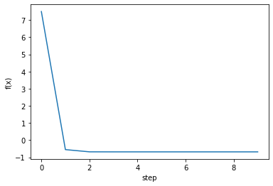
$8$ 번의 step 만에 $f(x)$를 최소로 만드는 해를 찾았다.

In [5]:

fig, ax = plt.subplots()
steps = np.arange(0, num_steps, 1)
fx = np.array([f(v) for v in history.T])
ax.plot(steps[:len(fx)], fx)
ax.set_xlabel('step')
ax.set_ylabel('f(x)')
plt.show()

Gradient Descent

In [6]:

def grad_decent(f, init, step, lr=0.001, history=False):
    
    def gradient(f, x, epsilon=1e-7):
        """ numerically find gradients. 
        x: shape=[n] """
        grad = np.zeros_like(x, dtype=float)
        for i in range(len(x)):
            h = np.zeros_like(x, dtype=float)
            h[i] = epsilon
            grad[i] = (f(x + h) - f(x - h)) / (2 * h[i])
        return grad
    
    x = deepcopy(init)
    memo = [x]
    for i in range(step - 1):
        # grad = gradient(f, x)
        grad = np.matmul(A, x) - b  # -graadient of f(x_i), of shape=[n]
        x = x - lr * grad
        if history: memo.append(x)
    if not history: return x
    return x, np.array(list(zip(*memo)))

In [7]:

num_steps = 2000
init = np.array([2, 1])
ans, history = grad_decent(f, init, step=num_steps, history=True)
print(f(init), f(ans))
print(ans)

7.5 -0.6817765890360808
[0.09416131 0.63143233]

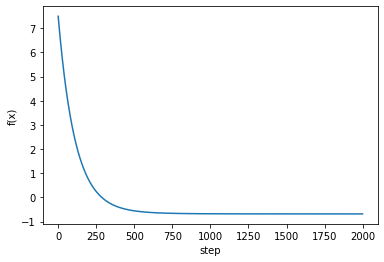
약 $500$ 번의 step 정도를 넘어야 $f$를 최소로 만드는 해를 찾았다, steepest descent 보다 느리다.

In [8]:

fig, ax = plt.subplots()
steps = np.arange(0, num_steps, 1)
fx = np.array([f(v) for v in history.T])
ax.plot(steps[:len(fx)], fx)
ax.set_xlabel('step')
ax.set_ylabel('f(x)')
plt.show()

Conjugate Gradient

conjugate gradient 방법은 $n \times n$ symetric, positive definite matrix $\mathbf{A}$에 대해
최적의 searching direction ($\mathbf{A}$ 의 conjugate vector들)과 line search (steepest descent에서의 방식을 이용한 learning rate 찾기)를 통해 $n$번의 업데이트 안에 앞서 정의한 $f(x)$의 최솟값, 즉 $\mathbf{A} \mathbf{x} = \mathbf{b}$의 해를 찾는 문제. 기본적으로 conjugate vector들을 momentum으로 사용하여 근사 해를 업데이트 해나간다.

$n \times n$ symetric, positive definite matrix $\mathbf{A}$ 이면

1. 최적의 searching direction이 conjugate vector들이 되는데 (linear algebra의 성질)이 $n$개의 conjugate vector들은 서로 orthogonal 해서, Gram-shmidt 과정을 통해 매 iteration마다 하나씩 구할 수 있다.
2. line search를 steepest descent방식과 유사하게 결정할 수있다.

참고이론: Cholesky decomposition

• Hermintian ($\mathbf{A} = \mathbf{A}^{*}$, 여기서 $\mathbf{A}^{*}$는 conjugate transpose)
• positive definite matrix ($\mathbf{x}^T\mathbf{A}\mathbf{x} > 0$)

인 경우 다음과 같은 cholesky decomposition 이 unique한 실수 행렬 $\mathbf{L}$을 갖는다.
\(\mathbf{A} = \mathbf{L} \mathbf{L}^* = \mathbf{L} \mathbf{L}^T, \text{where }\mathbf{L} \text{ is a lower triangular matrix with real and positive diagonal entries}\) LU 분해 보다 약 2배 가량 빠르다고 한다.

이를 이용하여 conjugate vector set을 생각할 수 있고, 이 벡터들을 찾아 n번의 업데이트 안에 해를 찾을 수 있음을 보일 수 있다.

잘 이해가 되지 않아 나중에 차근히 보도록 하겠다.

Procedure

$ - \nabla f(\mathbf{x}_i) = \mathbf{b} - \mathbf{A} \mathbf{x}_i$ 를 잔차 $\mathbf{r}_i$ 로 두고,
conjugate vector들을 $\mathbf{p}_1, \mathbf{p}_2, …, \mathbf{p}_n$ 이라 하자.

초기조건

• $\mathbf{p}_0$ = $\mathbf{r}_0$: 처음 잔차와 conjugate vector는 동일

1. Line Search

• update estimate
  steepest descent 에서 learning rate찾은 과정 이용
  recurrence 는 다음과 같다. \(\mathbf{x}_{i + 1} = \mathbf{x}_{i} + \alpha_{i} \mathbf{p}_i\)

이때, $\frac{\partial f(x_{i + 1})}{\partial \alpha_{i}} = 0$ 이용하여 $\alpha_i$ 결정.

\[\begin{align} \alpha_{i} &= \frac{\mathbf{p}_i^T (\mathbf{b} - \mathbf{A} \mathbf{x}_i)}{ \mathbf{p}_i^T \mathbf{A} \mathbf{p}_i} \\ &= \frac{\mathbf{p}_i^T \mathbf{r}_i}{ \mathbf{p}_i^T \mathbf{A} \mathbf{p}_i} \end{align}\]

• update residual
  

\[\begin{align} \mathbf{r}_{i + 1} &= \mathbf{b} - \mathbf{A} \mathbf{x}_{i + 1} \\ &= \mathbf{b} - \mathbf{A}(\mathbf{x}_i + \alpha_{i} \mathbf{p}_{i}) \\ &= (\mathbf{b} - \mathbf{A} \mathbf{x_i}) - \alpha_{i} \mathbf{A} \mathbf{p}_{i} \\ &= \mathbf{r}_i - \alpha_{i} \mathbf{A} \mathbf{p}_{i} \end{align}\]

2. Update search direction (Gram-schmidt on residual)

conjugate vector의 orthogonal한 성질을 이용해 찾는다. 

\[\begin{align} \mathbf{p}_{i + 1} &= \mathbf{r}_{i + 1} - \sum_{k \le i}{\frac{ \mathbf{r}_{i + 1}^T \mathbf{A} \mathbf{p}_k}{\mathbf{p}_k^{T} \mathbf{A} \mathbf{p}_k}} \mathbf{p}_{i} \\ &= \mathbf{r}_{i + 1} - \frac{ \mathbf{r}_{i + 1}^T \mathbf{A} \mathbf{p}_k}{\mathbf{p}_{i}^{T} \mathbf{A} \mathbf{p}_{i}} \mathbf{p}_{i}, \text{ since } \mathbf{p}_k^{T} \mathbf{A} \mathbf{r}_{i + 1} = 0, \forall k < i, \text{ conjugate vector의 성질} \\ &= \mathbf{r}_{i + 1} + \beta_{i} \mathbf{p}_i \end{align}\]

3. 반복

$\vert \alpha \mathbf{p}_i \vert$ 의 크기가 일정 bound보다 작아질때까지 1, 2를 반복한다.

$\alpha_i$ 와 $\beta_i$ wikipdia 표현으로 유도.

\[\begin{align} \alpha_i &= \frac{\mathbf{p}_i^T \mathbf{r}_i}{\mathbf{p}_i^T \mathbf{A} \mathbf{p}_i} \\ &= \frac{\mathbf{r}_i^T \mathbf{r}_i}{\mathbf{p}_i^T \mathbf{A} \mathbf{p}_i}, \text{ since } \mathbf{p}_i \mathbf{r}_i = \mathbf{r_i} \mathbf{r_i}, \text{from } \mathbf{p}_{i} = \mathbf{r}_{i} - \sum_{k < i}{\frac{ \mathbf{r}_{i}^{T} \mathbf{A} \mathbf{p}_k}{\mathbf{p}_k^{T} \mathbf{A} \mathbf{p}_k}} \mathbf{p}_{i - 1} \end{align}\] \[\require{cancel} \begin{align} \beta_i &= -\frac{\mathbf{r}_{i + 1}^T \mathbf{A} \mathbf{p}_i}{\mathbf{p}_i \mathbf{A} \mathbf{p}_{i}} \\ &= -\frac{\mathbf{r}_{i + 1}^T (\mathbf{r}_{i + 1} - \mathbf{r}_{i})}{\alpha \mathbf{p}_i \mathbf{A} \mathbf{p}_{i}} \text{, since } \mathbf{r}_{i + 1} = \mathbf{r}_i - \alpha_i \mathbf{A} \mathbf{p}_i \rightarrow \mathbf{A} \mathbf{p}_i = \frac{-(\mathbf{r}_{i + 1} - \mathbf{r}_i)}{\alpha} \\ &= \frac{\mathbf{r}_{i + 1}^T(\mathbf{r}_{i + 1} - \mathbf{r}_i)}{\frac{\mathbf{r}_i^T \mathbf{r}_i}{\cancel{\mathbf{p}_i^T\mathbf{A}\mathbf{p}_i}}\cancel{\mathbf{p}_i^T\mathbf{A}\mathbf{p}_i}} = \frac{\mathbf{r}_{i + 1}^T(\mathbf{r}_{i + 1} - \mathbf{r}_i)}{\mathbf{r}_i^T \mathbf{r}_i} \\ &= \frac{\mathbf{r}_{i + 1}^T \mathbf{r}_{i + 1}}{\mathbf{r}_i^T \mathbf{r}_i} \text{, since } \mathbf{r}_{i + 1}^T \mathbf{r}_{i} = 0 \end{align}\]

Implementation of CG

In [9]:

def conjugate(A, b, init, step, history=False):
    x = deepcopy(init)
    memo = [x]
    bound = 1e-7
    r = b - np.matmul(A, x)  # -graadient of f(x_i), of shape=[n]
    p = deepcopy(r) # inital search direction
    
    while step - 1:
        # line search
        pap = np.matmul(np.matmul(p.T, A), p)  # scalar
        alpha = np.matmul(r.T, r) / pap  # scalar
        
        # update estimate 
        x = x + alpha * p  # [n]
        if bound > sum(np.abs(alpha * p)): break
        
        # update residual and search direction
        r_prev = deepcopy(r)
        r = b - np.matmul(A, x)

        # r = r - np.matmul(alpha * A, p)  # [n]
        # beta = np.matmul(np.matmul(r.T, A), p) / pap  # scalar
        beta = np.matmul(r.T, r) / np.matmul(r_prev.T, r_prev)
        p = r + beta * p  # [n]
        if history: memo.append(x)
        step -= 1
    if not history: return x
    return x, np.array(list(zip(*memo)))

In [10]:

num_steps = 100
init = np.array([2, 1], dtype=float)
ans, history = conjugate(A, b, init, step=num_steps, history=True)
print(f(init), f(ans))
print(ans)

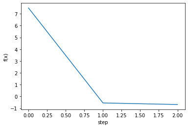
7.5 -0.6818181818181818
[0.09090909 0.63636364]

In [11]:

fig, ax = plt.subplots()
steps = np.arange(0, num_steps, 1)
fx = np.array([f(v) for v in history.T])
ax.plot(steps[:len(fx)], fx)
ax.set_xlabel('step')
ax.set_ylabel('f(x)')
plt.show()

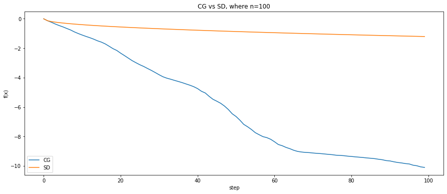
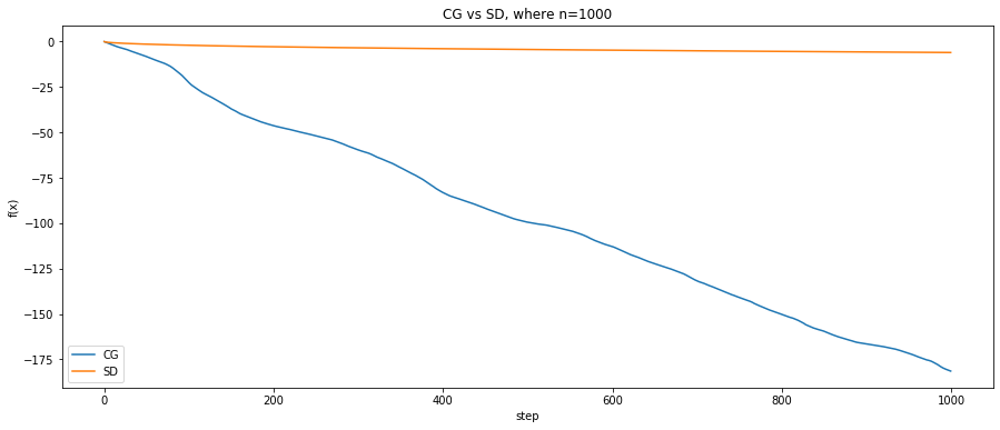
Experiments

In [12]:

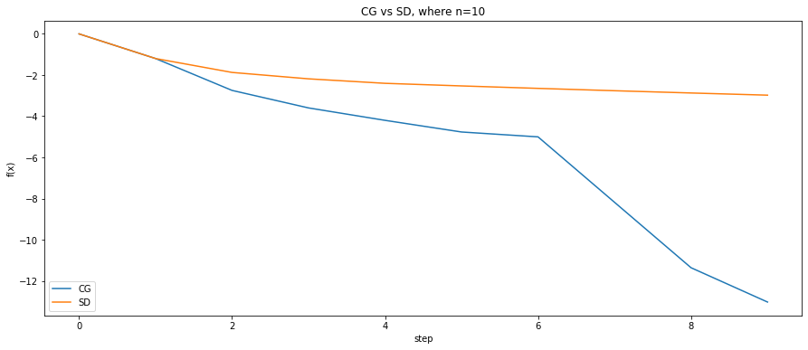
for k, n in enumerate([10, 100, 1000]):
    P = np.random.normal(size=[n, n])
    A = np.dot(P.T, P)
    b = np.random.rand(n)
    num_steps = n
    
    def f(x):
        """ x is a vector, of shape=[n]"""
        return (1 / 2) * np.matmul(np.matmul(x.T, A), x) - np.matmul(b.T, x) 

    init = np.zeros(n)
    ans1, history1 = conjugate(A, b, deepcopy(init), step=num_steps, history=True)
    ans2, history2 = steepest_grad_decent(A, b, deepcopy(init), step=num_steps, history=True)

    steps = np.arange(0, num_steps, 1)
    fx1 = np.array([f(v) for v in history1.T])
    fx2 = np.array([f(v) for v in history2.T])
    fig, ax = plt.subplots(nrows=1, ncols=1, figsize=(15, 6))
    ax.plot(steps[:len(fx1)], fx1, label='CG')
    ax.plot(steps[:len(fx2)], fx2, label='SD')
    ax.legend(loc='lower left')
    ax.set_xlabel('step')
    ax.set_ylabel('f(x)')
    ax.set_title('CG vs SD, where n={}'.format(n))
    plt.show()

Reference

[1] conjugate gradient paper
[2] hojoon’s blog korean
[3] slide korean
[4] comparision steepest descent vs conjugate gradient
[5] standford cs 205 tutorial, chaptor 10
[6] english tutorial