Implementation of Gaussian HMM

Hidden Markov Model under Continuous Observation

기존의 HMM은 discrete observation에 대해서만 적용이 가능했다. 만약 continous observation에서 HMM을 적용하려면 어떻게 해야할까?
observation을 Gaussian Variable로 모델링하면 된다. 그러면 각 state별로 평균과 분산에 대한 파라미터를 추정한다면 위의 문제를 풀 수 있게된다.
예를 들어, hot/cold state에서 온도를 관측한다고 하자.
관측값은 $P(\mu_{1}, \sigma_{1} \vert hot)$ 과 $P(\mu_{2}, \sigma_{2} \vert cold)$ 의 두 분포중 하나에 속하게 될 것이다.
두 분포의 확률을 각각 방출확률로 추정한다면 discrete observation을 continuous observation으로 확장할 수 있다.
reference

In [1]:

import numpy as np
import seaborn as sns
import matplotlib.pyplot as plt

from hmmlearn.hmm import GaussianHMM

np.set_printoptions(precision=3, suppress=True)

Define Model

In [2]:

model = GaussianHMM(n_components=2, covariance_type="diag")
model.startprob_ = np.array([0.9, 0.1])
model.transmat_ = np.array([[0.95, 0.05], [0.15, 0.85]])
model.means_ = np.array([[5.0], [-10.0]])
model.covars_ = np.array([[15.0], [40.0]])

Generate Samples

In [3]:

X, Z = model.sample(1000)
X.shape, Z.shape

((1000, 1), (1000,))

Visualize Distribution of Samples

In [4]:

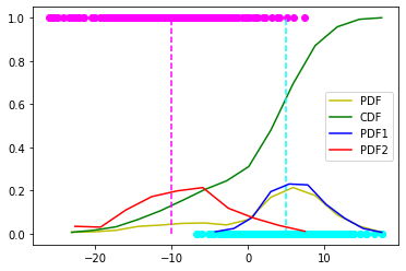
count, bins_count = np.histogram(X, bins=15)
pdf = count / sum(count)
# using numpy np.cumsum to calculate the CDF
# We can also find using the PDF values by looping and adding
cdf = np.cumsum(pdf)
# plotting PDF and CDF
plt.plot(bins_count[1:], pdf, color="y", label="PDF")
plt.plot(bins_count[1:], cdf, color="g", label="CDF")
plt.vlines(x=5, ymin=0, ymax=1.0, color='cyan', ls='--')
plt.vlines(x=-10, ymin=0, ymax=1.0, color='magenta', ls='--')

mask = Z == 0

count, bins_count = np.histogram(X[mask], bins=10)
pdf = count / sum(count)
plt.plot(bins_count[1:], pdf, color="b", label="PDF1")

count, bins_count = np.histogram(X[~mask], bins=10)
pdf = count / sum(count)
plt.plot(bins_count[1:], pdf, color="r", label="PDF2")

plt.scatter(X[mask], Z[mask], color='cyan')
plt.scatter(X[~mask], Z[~mask], color='magenta')
plt.legend()

<matplotlib.legend.Legend at 0x7f018c473e90>

In [5]:

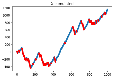
X_cumsum = X.cumsum()
X_cumsum_hat = X_cumsum.copy()
X_cumsum_hat[mask] = np.nan
plt.plot(X_cumsum, lw=5)
plt.plot(X_cumsum_hat, 'r-', lw=5)
plt.title("X cumulated")

Text(0.5, 1.0, 'X cumulated')

Train Model

In [6]:

trained_model = GaussianHMM(n_components=2, n_iter=len(X), verbose=True, tol=1e-10)
print("initial model parameters:\n"
f'startprob : {trained_model.startprob_prior}\n' 
f'transmat_: {trained_model.transmat_prior}\n' 
f'means: {trained_model.means_prior}\n' 
f'covars: {trained_model.covars_prior}\n')

trained_model.fit(X)

print("GT model parameters:\n"
f'startprob : {model.startprob_}\n'
f'transmat_: {model.transmat_}\n' 
f'means: {model.means_}\n' 
f'covars: {model.covars_}\n')

print("final model parameters:\n"
f'startprob : {trained_model.startprob_}\n'
f'transmat_: {trained_model.transmat_}\n' 
f'means: {trained_model.means_}\n' 
f'covars: {trained_model.covars_}\n')

initial model parameters:
startprob : 1.0
transmat_: 1.0
means: 0
covars: 0.01

GT model parameters:
startprob : [0.9 0.1]
transmat_: [[0.95 0.05]
 [0.15 0.85]]
means: [[  5.]
 [-10.]]
covars: [[[15.]]

 [[40.]]]

final model parameters:
startprob : [1. 0.]
transmat_: [[0.948 0.052]
 [0.142 0.858]]
means: [[ 5.174]
 [-9.955]]
covars: [[[15.173]]

 [[41.75 ]]]

         1       -3668.0490             +nan
         2       -3298.6730        +369.3759
         3       -3174.2007        +124.4723
         4       -3134.2000         +40.0007
         5       -3129.1966          +5.0034
         6       -3128.6905          +0.5061
         7       -3128.6226          +0.0679
         8       -3128.6108          +0.0118
         9       -3128.6085          +0.0023
        10       -3128.6080          +0.0005
        11       -3128.6079          +0.0001
        12       -3128.6079          +0.0000
        13       -3128.6079          +0.0000
        14       -3128.6079          +0.0000
        15       -3128.6079          +0.0000
        16       -3128.6079          +0.0000
        17       -3128.6079          +0.0000
        18       -3128.6079          +0.0000
        19       -3128.6079          +0.0000
        20       -3128.6079          +0.0000
        21       -3128.6079          +0.0000

Test

In [7]:

X, Z = model.sample(1000)
Z_hat = trained_model.predict(X)
accuracy = (Z == Z_hat).sum() / len(Z)
accuracy = 1 - accuracy if accuracy < 0.5 else accuracy
print(f'accuracy : {accuracy*100:<.3f} %')

accuracy : 98.500 %