
In [1]:
1
2
3
4
5
6
7
8
9
import torch
import numpy as np
import matplotlib.pyplot as plt
from matplotlib.colors import ListedColormap

from hmmlearn.hmm import GaussianHMM

np.set_printoptions(precision=3, suppress=True)
%matplotlib inline
In [2]:
1
2
3
4
data_path = 'data/train.pt'
data = torch.load(data_path)
N, C, T, V = data.shape
data.shape
1
torch.Size([67718, 10, 24, 10])
In [3]:
1
2
3
4
N = 500
num_states = 3
data = data[np.random.choice(range(N), N)]
data.shape
1
torch.Size([500, 10, 24, 10])
In [4]:
1
2
3
4
5
num_objects = data[:,-1,-1].sum(1).numpy().astype(int)
X = torch.cat([data[i,:-1,:,:n].permute(2,1,0) for i, n in enumerate(num_objects)]).numpy() # N, T, C
L = np.array(X.shape[0] * [X.shape[1]])
X = X.reshape(-1, C-1)
X.shape, L
1
((41616, 9), array([24, 24, 24, ..., 24, 24, 24]))
In [5]:
1
2
3
trained_model = GaussianHMM(n_components=num_states, n_iter=N*10, verbose=True, tol=1e-10)

trained_model.fit(X, L)
1
2
3
4
5
6
7
8
9
10
11
12
13
14
15
16
17
18
19
20
21
22
23
24
25
26
27
28
29
30
31
32
33
34
35
36
37
38
39
40
41
42
43
44
45
46
47
48
49
50
51
         1     -662674.4627             +nan
         2     -612362.9883      +50311.4744
         3     -527996.5661      +84366.4221
         4     -386087.2248     +141909.3413
         5     -288414.5388      +97672.6860
         6     -249723.9687      +38690.5701
         7     -197032.9378      +52691.0309
         8     -167593.5663      +29439.3715
         9     -161980.5326       +5613.0337
        10     -156040.2651       +5940.2675
        11     -151346.2949       +4693.9702
        12     -148383.1823       +2963.1126
        13     -146283.8510       +2099.3312
        14     -144802.7061       +1481.1449
        15     -144227.5810        +575.1252
        16     -144008.0702        +219.5108
        17     -143867.5950        +140.4751
        18     -143758.8215        +108.7735
        19     -143648.9633        +109.8583
        20     -143540.6495        +108.3138
        21     -143454.9027         +85.7468
        22     -143385.5742         +69.3285
        23     -143325.1282         +60.4460
        24     -143281.5400         +43.5881
        25     -143239.9319         +41.6081
        26     -143223.1078         +16.8242
        27     -143216.6505          +6.4573
        28     -143211.7679          +4.8826
        29     -143193.3477         +18.4202
        30     -143106.4029         +86.9448
        31     -142936.8979        +169.5049
        32     -142763.5685        +173.3294
        33     -142628.3667        +135.2018
        34     -142565.2359         +63.1308
        35     -142519.8133         +45.4226
        36     -142380.2397        +139.5736
        37     -141846.5114        +533.7283
        38     -141551.8564        +294.6550
        39     -141325.3312        +226.5252
        40     -140950.6366        +374.6946
        41     -140722.0542        +228.5824
        42     -140282.7640        +439.2901
        43     -138684.5387       +1598.2253
        44     -135834.9579       +2849.5808
        45     -135793.9120         +41.0458
        46     -135778.4024         +15.5096
        47     -135772.6509          +5.7515
        48     -135770.8351          +1.8157
        49     -135770.4953          +0.3398
        50     -135770.6152          -0.1199
1
GaussianHMM(n_components=3, n_iter=5000, tol=1e-10, verbose=True)
In [6]:
1
2
3
4
5
print("Final Model Parameters:\n"
f'\tstartprob : {trained_model.startprob_}\n'
f'\ttransmat_: {trained_model.transmat_}\n'
f'\tmeans: {trained_model.means_}\n'
f'\tcovars: {[np.diag(cov) for cov in trained_model.covars_]}\n')
1
2
3
4
5
6
7
8
9
10
11
12
13
14
Final Model Parameters:
	startprob : [0.641 0.215 0.145]
	transmat_: [[0.975 0.022 0.004]
 [0.048 0.93  0.022]
 [0.002 0.021 0.977]]
	means: [[19.28   1.088  0.002  0.005  0.304  0.008  0.265 -0.002  0.   ]
 [14.999  2.536  0.814  3.223 -0.316  0.069 -0.174  0.     0.   ]
 [20.497 -5.339 -0.973  1.666 -2.324 -0.065 -0.433 -0.014  0.001]]
	covars: [array([204.865,   2.673,   0.   ,   0.001,   7.092,   0.002,  26.902,
         0.   ,   0.   ]), array([492.609,   3.587,   2.784,  29.518,   7.126,   0.129,  14.481,
         0.   ,   0.   ]), array([278.487, 206.211,   7.345,  27.703,  22.276,   9.471,   9.437,
         0.016,   0.003])]
Test and Visualize
In [7]:
1
2
3
4
5
6
7
8
9
10
11
12
13
# data_path = 'data/test.pt'
# data = torch.load(data_path)
# N, C, T, V = data.shape

# N = 500
# num_states = 3
# data = data[np.random.choice(range(N), N)]

# num_objects = data[:,-1,-1].sum(1).numpy().astype(int)
# X = torch.cat([data[i,:-1,:,:n].permute(2,1,0) for i, n in enumerate(num_objects)]).numpy() # N, T, C
# L = np.array(X.shape[0] * [X.shape[1]])
# X = X.reshape(-1, C-1)
# X.shape, L
In [8]:
1
Z = trained_model.predict(X, L)
In [9]:
1
2
3
cum_objects = np.insert(np.cumsum(num_objects), 0, 0)
predicted_states = [Z.reshape(-1, T)[cum_objects[idx]:cum_objects[idx+1]] for idx in range(N)]
len(predicted_states), predicted_states[0].shape, data.shape
1
(500, (3, 24), torch.Size([500, 10, 24, 10]))
In [128]:
1
2
3
4
5
6
7
8
9
10
11
12
13
14
15
16
17
18
19
20
21
22
23
24
25
26
27
28
29
30
31
32
33
34
35
36
37
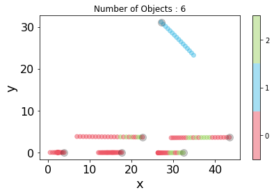
colorlist = ['#ED5564', '#4FC1E8', '#A0D568'] #, '#FFCE54', '#AC92EB'
cmap = ListedColormap(colorlist)
sample_idx = int(np.random.choice(range(N), 1))
sample = data[sample_idx, [0,1,-1]].numpy()
predict = predicted_states[sample_idx]
num_obj = int(sample[-1,-1,:].sum())
sample = np.transpose(sample, (2,1,0))[:num_obj] # (V, T, C)
for history, state in zip(sample, predict):
mask = history[:,-1] == 1
history = history[mask]
# plt.scatter(history[:,0], history[:,1], c='k', alpha=0.1)
# plt.scatter(history[-1,0], history[-1,1], c='cyan', alpha=1.0)
im = plt.scatter(history[:,0], history[:,1], c=state[mask], cmap=cmap, alpha=0.5)
plt.scatter(history[-1,0], history[-1,1], c='k', s=100, alpha=0.2)
ax = plt.gca()
limits=plt.axis('on') # turns on axis
ax.tick_params(left=True, bottom=True, labelleft=True, labelbottom=True)
ax.tick_params('x',labelsize=16)
ax.tick_params('y',labelsize=16)
ax.set_xlabel('x', fontsize=18)
ax.set_ylabel('y', fontsize=18)
plt.title(f'Number of Objects : {num_obj}')
plt.axis('equal')
plt.tight_layout()
cbar = plt.colorbar(im)
offset = (cbar.vmax - cbar.vmin) / (2 * num_states)
tick_locs = np.linspace(cbar.vmin, cbar.vmax, num_states + 1)[:-1] + offset
cbar.set_ticks(tick_locs)
cbar.set_ticklabels(np.arange(num_states))
plt.show()

Leave a comment