
1
2
3
4
5
6
import numpy as np
import matplotlib.pyplot as plt
from copy import deepcopy
from mpl_toolkits import mplot3d
from math import cos, sin, exp
np.set_printoptions(precision=6)
Newton Raphson Method (with Implementation)
일반적인 설명: 해를 쉽게 구할 수 없는 고차원의 $f(x)$가 주어지면, $f(x) = 0$ 의 해를 임의의 초깃값으로부터 점진적으로(수치해석적으로) 구한다. wiki
활용: $f(x) = 0$ 를 구한다는 말은 임의의 음함수 $f(x1, x2, …, x_n) = f(\mathbf{x}) = 0$ 를 구한다고 할 수 있고 ($\mathbf{x}$는 벡터표현)
벡터로 생각하면, 음함수 및 연립 방정식도 생각 가능하다.
또한, 최소/최대 값을 구할 때에도 $f’(\mathbf{x}) = 0$의 해를 구하므로써 최소/최대 값이 되는 $\mathbf{x}$를 구할 수 있다.
Idea: How to find a solution numerically?
Toy example을 풀기 전 일반적으로 $f(x) = 0$을 찾는 과정을 설명하겠다.
임의의 초깃값에 대한 접선으로부터 $x$ intercept(x 축과의 교점)으로 이동하고, 같은 과정을 반복한다.
\[\begin{align} y &= f'(x_i)(x - x_i) + f(x_i) \\ 0 &= f'(x_i)(x_{i + 1} - x_i) + f(x_i) \\ \therefore x_{i+1} = x_i -\frac{f(x_i)}{f'(x_i)} &\underset{\text{vector representation}}{\Longleftrightarrow} \mathbf{x}_{i + 1} = \mathbf{x}_i - \mathbf{J}^{-1}(f(\mathbf{x}_i))f(\mathbf{x}_i)\\ \end{align}\]위의 업데이트 과정을 수렴할때까지 반복
Math
-
First derivative
- gradient: 각 차원별 1차 미분, 벡터가 됨
- jacobian: 서로 다른 차원 사이 1차 미분(input 차원 $n$, output의 차원 $m$ 이라면 $m \times n$ matrix)
- Second derivative
- hessian: 서로 다른 차원 사이 곡률(curvature)특성을 나타낸 2차 미분 $n \times n$ matrix
- laplacian 각 차원 2차 미분값의 합, scalar
나중에 선형대수 편을 정리하겠다.
Example 1
다양한 상황 이해를 위해, multi-variable, $f: \mathbb{R}^3 \rightarrow \mathbb{R}^3$ 인 상황인 문제를 풀겠다.
detail을 알고싶다면 [3]참조.
특히 연립방정식에 대한 Newton Rapshon 방식을 Gauss-Newton 방식이라고 부른다.
주의할 점은 업데이트 하는 recurrence에서 jacobian의 inverse가 존재하지 않을 때는
다음 식과 같이 pseudo inverse를 활용한다. (만약 $\mathbf{J}^T \mathbf{J}$에 대한 inverse도 존재하지 않는 경우에는 해를 구할 수 없다.)
\(\mathbf{x}_{i + 1} = \mathbf{x}_i - (\mathbf{J}^{T} \mathbf{J})^{-1}\mathbf{J}^T f(\mathbf{x}_i)\)
내가 구현한 방식은 simple한 문제를 풀기 위해 $\mathbf{J}$의 역행렬이 존재하지 않아 pseudo inverse를 이용하는 경우에 대한 코딩은 생략하였다.
다음과 같은 예제를 풀어보자.
\[\begin{align} \begin{cases} 3x_1 - cos(x_2x_3) - 3/2 = 0 \\ 4x_1^2 - 625x_2^2 + 2x_3 - 1 = 0 \\ 20x_3 + e^{-x_1x_2} + 9 = 0\\ \end{cases} \end{align}\]1
2
3
4
5
6
7
def f(x):
f1 = 3 * x[0] - cos(x[1] * x[2]) - 3 / 2
f2 = 4 * (x[0] ** 2) - 625 * (x[1] ** 2) + 2 * x[2] - 1
f3 = 20 * x[2] + exp(-x[0] * x[1]) + 9
return f1, f2, f3
f([1, 1, 1])
1
(0.9596976941318602, -620, 29.367879441171443)
Step 1. First Derivative: Gradient or Jacobian
1
2
3
4
5
6
7
8
9
10
11
12
13
14
def gradient(f, x, epsilon=1e-7):
    """ numerically find gradients.
    x: shape=[2] """
    grad = np.zeros_like(x, dtype=float)
    for i in range(len(x)):
        h = np.zeros_like(x, dtype=float)
        h[i] = epsilon
        grad[i] = (f(x + h) - f(x - h)) / (2 * h[i])
    return grad

m = 3  # for f1, f2, f3
x = [1, 1, 1]
for i in range(m):
    print(gradient(lambda e: f(e)[i], x))
1
2
3
4
[3.       0.841471 0.841471]
[    8. -1250.     2.]
[-0.367879 -0.367879 20.      ]
1
2
3
4
5
6
7
8
9
10
11
12
13
14
15
16
17
18
19
20
def jacobian(f, m, x, epsilon=1e-7):
    """ numerically find gradients.
    f: shape=[m]
    x: shape=[n] """

    def gradient(f, x, epsilon=1e-7):
        """ numerically find gradients.
        x: shape=[n] """
        grad = np.zeros_like(x, dtype=float)
        for i in range(len(x)):
            h = np.zeros_like(x, dtype=float)
            h[i] = epsilon
            grad[i] = (f(x + h) - f(x - h)) / (2 * h[i])
        return grad

    jaco = np.zeros(shape=(m, len(x)), dtype=float)
    for i in range(m):
        jaco[i, :] = gradient(lambda e: f(e)[i], x)

    return jaco
1
2
3
m = 3
init = [1, 1, 1]
jacobian(f, m, init)
1
2
3
array([[ 3.000000e+00,  8.414710e-01,  8.414710e-01],
       [ 8.000000e+00, -1.250000e+03,  2.000000e+00],
       [-3.678794e-01, -3.678794e-01,  2.000000e+01]])
Forward one step
1
2
3
4
5
x = init
J_inv = np.linalg.inv(jacobian(f, m, x))
update = np.matmul(J_inv, f(x))
x = x - update
init, x
1
([1, 1, 1], array([ 1.232701,  0.503132, -0.473253]))
1
2
3
4
5
6
7
8
9
10
11
12
13
14
15
16
17
18
19
def newton(f, m, init, epsilon=1e-7, verbose=True, history=False):
    """ Newton Raphson Method.
    f: function
    m: the number of output dimension
    init: np.array, with dimension n """
    x = deepcopy(init)
    bound = 1e-7
    memo = [x]
    while True:
        assert m == len(x), "inverse of jacobian does not exist"
        J_inv = np.linalg.inv(jacobian(f, m, x))
        update = np.matmul(J_inv, f(x))
        x = x - update
        if bound > sum(np.abs(update)):
            break
        if verbose: print("x={} update={}".format(x, sum(np.abs(update))))
        if history: memo.append(x)
    if not history: return x
    return x, np.array(list(zip(*memo)))
1
2
ans = newton(f, m=3, init=np.array([1, 1, 1]), verbose=True)
ans
1
2
3
4
5
6
7
8
9
x=[ 1.232701  0.503132 -0.473253] update=2.202821628129451
x=[ 0.832592  0.251806 -0.490636] update=0.6688171563971012
x=[ 0.833238  0.128406 -0.494702] update=0.12811189204889828
x=[ 0.833275  0.069082 -0.497147] update=0.0618067785892694
x=[ 0.833281  0.043585 -0.498206] update=0.026560726591480517
x=[ 0.833282  0.036117 -0.498517] update=0.0077800841534735096
x=[ 0.833282  0.035343 -0.498549] update=0.0008059062665949748
x=[ 0.833282  0.035335 -0.498549] update=8.83724325344356e-06
1
array([ 0.833282,  0.035335, -0.498549])
1
f(ans)
1
(-4.440892098500626e-16, -8.881784197001252e-16, 0.0)
Example 2
\(\begin{align} \begin{cases} x_1 - 2x_1 + x_2^2 - x_3 + 1 = 0 \\ x_1x_2^2 - x_1 - 3x_2 + x_2x_3 + 2 = 0\\ x_1x_3^2 - 3x_3 + x_2x_3^2 + x_1x_2 = 0\\ \end{cases} \end{align}\)
1
2
3
4
5
def f(x):
    f1 = x[0]**2 - 2 * x[0] + x[1] ** 2 - x[2] + 1
    f2 = x[0] * (x[1] ** 2) - x[0] - 3 * x[1] + x[1] * x[2] + 2
    f3 = x[0] * (x[2] ** 2) - 3 * x[2] + x[1] * (x[2] ** 2) + x[0] * x[1]
    return f1, f2, f3
1
2
ans = newton(f, m=3, init=[1, 2, 3], verbose=True)
ans
1
2
3
4
5
6
7
8
9
10
x=[0.102564 1.641026 2.564103] update=1.6923076937371369
x=[1.520623 1.411129 0.19859 ] update=4.013468189506828
x=[1.941234 0.771343 0.894651] update=1.756458358638363
x=[1.067366 1.191171 0.483526] update=1.7048211972702223
x=[1.268254 0.951822 0.880281] update=0.8369921098348203
x=[0.958988 1.033836 0.968126] update=0.4791268413760061
x=[1.001713 1.00007  0.997178] update=0.10554262942044743
x=[1.000001 1.000001 1.      ] update=0.004602265817081868
x=[1. 1. 1.] update=3.035297397391498e-06
1
array([1., 1., 1.])
1
2
ans = newton(f, m=3, init=[0, 0, 0], verbose=True)
ans
1
2
3
4
5
6
7
8
9
x=[0.5 0.5 0. ] update=1.0000000000637628
x=[0.839506 0.475309 0.135802] update=0.500000000431082
x=[0.985821 0.418485 0.150694] update=0.21802966946639207
x=[1.054172 0.387153 0.147169] update=0.10320806798316114
x=[1.085652 0.373392 0.145578] update=0.04683201152930883
x=[1.096933 0.368489 0.145029] update=0.01673402200201663
x=[1.098881 0.367643 0.144935] update=0.002887003029724366
x=[1.098943 0.367617 0.144932] update=9.147370504047642e-05
1
array([1.098943, 0.367617, 0.144932])
Example 3
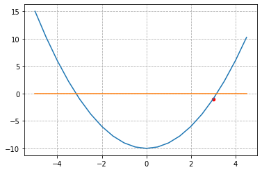
\[\begin{align} f(x) &= x^2 - 10 \\ 0 &= x^2 - 10 \\ x &= \pm \sqrt{10} \\ \end{align}\]1
2
3
4
5
6
7
8
9
10
11
12
13
14
15
def f(x):
return x ** 2 - 10
x = np.arange(-5, 5, 0.5)
y = f(x)
hyperplane = np.zeros_like(x)
print(x.shape, y.shape)
fig = plt.figure()
ax = plt.axes()
ax.plot(x, y)
ax.plot(x, hyperplane)
ax.scatter([3], [f(3)], s=20, color='red')
plt.grid(linestyle='--')
plt.show()
1
2
(20,) (20,)
1
2
ans = newton(f, m=1, init=np.array([3]), verbose=True)
ans
1
2
3
4
x=[3.166667] update=0.1666666669394298
x=[3.162281] update=0.004385965191196533
x=[3.162278] update=3.0415783977039912e-06
1
array([3.162278])
Example 4
1
2
3
4
5
6
7
8
9
10
11
12
13
14
15
16
17
18
19
20
21
22
23
24
25
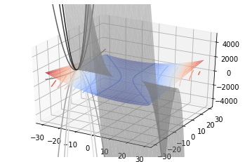
x1 = np.arange(-30, 30, 1)
x2 = np.arange(-30, 30, 1)
print(x1.shape, x2.shape)
x1, x2 = np.meshgrid(x1, x2) # outer product by ones_like(x1) or ones_like(x2)
def f(x):
f1 = x[0]**2 - 2 + x[0]*x[1] - 10
f2 = x[1]**2 - 3*x[0]*(x[1]**2) - 57
return f1, f2
x = np.concatenate((x1[np.newaxis, :], x2[np.newaxis, :]), axis=0)
print(x[0].shape, x[1].shape)
y = np.array(f(x))
hyperplane = np.zeros_like(x1)
print(x1.shape, x2.shape, y.shape)
fig = plt.figure()
ax = plt.axes(projection='3d')
ax.plot_surface(x1, x2, y[0], cmap='coolwarm', alpha=0.7)
ax.contour(x1, x2, y[0], cmap='coolwarm', offset=0, alpha=1)
ax.plot_surface(x1, x2, y[1], cmap='gray', alpha=0.5)
ax.contour(x1, x2, y[1], cmap='gray', zdir='x', offset=-30, alpha=1)
# ax.plot_surface(x1, x2, hyperplane, alpha=0.5)
ax.set_zlim(-5000, 5000)
plt.show()
1
2
3
4
(60,) (60,)
(60, 60) (60, 60)
(60, 60) (60, 60) (2, 60, 60)
1
2
3
4
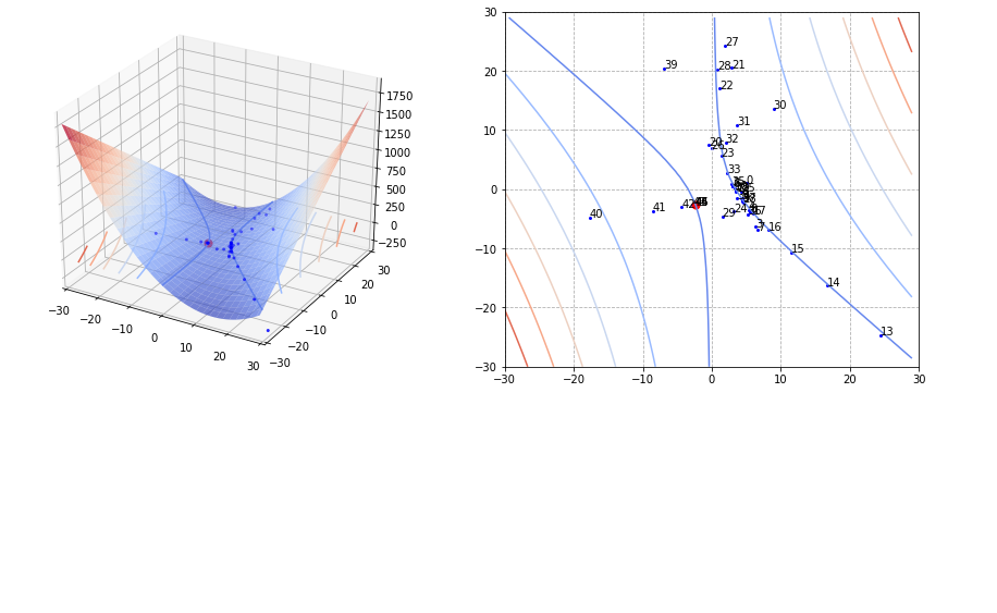
ans, history = newton(f, m=2, init=np.array([5., 1.]), history=True)
print(history.shape)
print(ans)
print("f(ans) = {}".format(f(ans)))
1
2
3
4
5
6
7
8
9
10
11
12
13
14
15
16
17
18
19
20
21
22
23
24
25
26
27
28
29
30
31
32
33
34
35
36
37
38
39
40
41
42
43
44
45
46
47
48
49
50
x=[ 4.491468 -1.481229] update=2.9897610912892185
x=[3.073134 0.549184] update=3.4487469172444447
x=[ 6.378826 -6.370453] update=10.225330245654375
x=[ 5.358633 -3.47607 ] update=3.9145774809611384
x=[ 4.224355 -1.58649 ] update=3.0238571449006724
x=[3.059681 0.508261] update=3.259425753764904
x=[ 6.66039  -6.937257] update=11.046227634721145
x=[ 5.594116 -3.836744] update=4.166786219891734
x=[ 4.402018 -1.882414] update=3.146428860525024
x=[3.306956 0.045852] update=3.0233279503405157
x=[ 38.186497 -69.920943] update=104.84633614549777
x=[ 35.518073 -37.421387] update=35.16798054774894
x=[ 24.371564 -24.631017] update=23.936878558723713
x=[ 16.660407 -16.250121] update=16.092052372087466
x=[ 11.503055 -10.655777] update=10.751696797973349
x=[ 8.142025 -6.851262] update=7.165544652576577
x=[ 6.00073  -4.187433] update=4.805123679894626
x=[ 4.620288 -2.20339 ] update=3.3644855564382965
x=[ 3.537712 -0.374169] update=2.9117968229359312
x=[-0.498923  7.500642] update=11.91144500180123
x=[ 2.881338 20.504327] update=16.383946296526858
x=[ 1.155922 17.01272 ] update=5.217022997922324
x=[1.375131 5.560684] update=11.671245231046441
x=[ 3.215405 -3.770844] update=11.171802846740402
x=[ 4.24677  -0.336576] update=4.465633231448297
x=[-0.063991  6.858782] update=11.506119607818658
x=[ 1.949196 24.291654] update=19.446059618603222
x=[ 0.841096 20.232967] update=5.166787041731603
x=[ 1.531627 -4.566096] update=25.489593861668588
x=[ 8.944667 13.576908] update=25.55604516824303
x=[ 3.701962 10.840108] update=7.979505280438819
x=[2.008696 7.884326] update=4.649047869342555
x=[2.216521 2.733946] update=5.358205378379376
x=[ 3.682322 -1.542212] update=5.741959725544182
x=[2.858799 0.878633] update=3.2443684263338985
x=[ 5.287208 -4.264406] update=7.571447830261409
x=[ 4.465048 -2.036373] update=3.050193517755833
x=[ 3.410273 -0.149007] update=2.9421404118502865
x=[-6.959394 20.394751] update=30.9134248479969
x=[-17.704566  -4.763661] update=35.90358464317116
x=[-8.570734 -3.698475] update=10.199018089887751
x=[-4.385028 -3.007022] update=4.877158727279548
x=[-2.770593 -2.687522] update=1.9339352352799333
x=[-2.407191 -2.639919] update=0.4110045050978556
x=[-2.386085 -2.64323 ] update=0.024415772855854504
x=[-2.386016 -2.643287] update=0.00012616945083334416
(2, 47)
[-2.386016 -2.643287]
f(ans) = (1.7763568394002505e-15, 7.105427357601002e-15)
1
2
3
4
5
6
7
8
9
10
11
12
13
14
15
16
17
18
19
20
21
22
23
24
fig, (ax11, ax12) = plt.subplots(nrows=1, ncols=2, figsize=(15, 6))

""" f1 figure """
ax11.remove()
ax11 = fig.add_subplot(1,2,1,projection='3d')
ax11.plot_surface(x1, x2, y[0], cmap='coolwarm', alpha=0.7)
ax11.contour(x1, x2, y[0], cmap='coolwarm', zdir='z', offset=0, alpha=1)
ax11.scatter(history[0, :], history[1, :], s=4, color='blue')
ax11.scatter(*ans, s=50, color='red')
# ax1.plot(history[0, :], history[1, :], color='black', linewidth=0.5)
ax11.set_xlim(-30, 30), ax11.set_ylim(-30, 30)

order = list(range(len(history[0])))
ax12.contour(x1, x2, y[0], cmap='coolwarm', alpha=1)
ax12.scatter(history[0, :], history[1, :], s=4 ,color='blue')
order = list(range(len(history[0])))
for i, txt in enumerate(order):
    ax12.annotate(txt, (history[0][i], history[1][i]))
ax12.scatter(*ans, s=50, color='red')
# ax2.plot(history[0, :], history[1, :], color='black', linewidth=0.5)
ax12.set_xlim(-30, 30), ax12.set_ylim(-30, 30)
ax12.grid(linestyle='--')

plt.show()
1
2
3
4
5
6
7
8
9
10
11
12
13
14
15
16
17
18
19
20
21
22
23
24
25
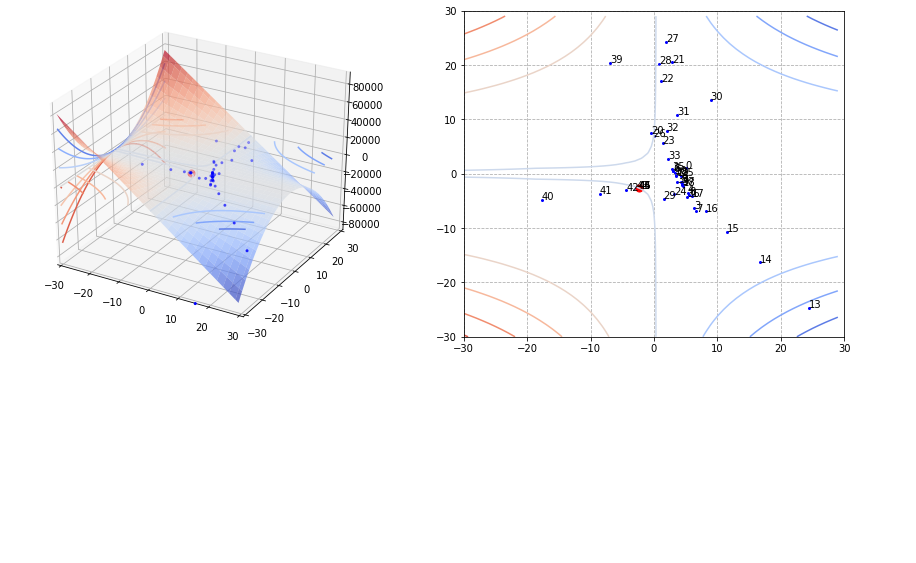
fig, (ax21, ax22) = plt.subplots(nrows=1, ncols=2, figsize=(15, 6))
""" f2 figure """
ax21.remove()
ax21 = fig.add_subplot(1,2,1,projection='3d')
ax21.plot_surface(x1, x2, y[1], cmap='coolwarm', alpha=0.7)
ax21.contour(x1, x2, y[1], cmap='coolwarm', zdir='z', offset=0, alpha=1)
ax21.contour(x1, x2, y[1], cmap='coolwarm', zdir='x', offset=-30, alpha=1)
ax21.scatter(history[0, :], history[1, :], s=4, color='blue')
ax21.scatter(*ans, s=50, color='red')
# ax1.plot(history[0, :], history[1, :], color='black', linewidth=0.5)
ax21.set_xlim(-30, 30), ax21.set_ylim(-30, 30)
order = list(range(len(history[0])))
ax22.contour(x1, x2, y[1], cmap='coolwarm', alpha=1)
ax22.scatter(history[0, :], history[1, :], s=4 ,color='blue')
order = list(range(len(history[0])))
for i, txt in enumerate(order):
ax22.annotate(txt, (history[0][i], history[1][i]))
ax22.scatter(*ans, s=50, color='red')
# ax2.plot(history[0, :], history[1, :], color='black', linewidth=0.5)
ax22.set_xlim(-30, 30), ax22.set_ylim(-30, 30)
ax22.grid(linestyle='--')
plt.show()
Furthermore
최소/최대값을 구할때는 $f’(x) = 0$ 의 해를 찾는 것이므로 다음과 같은 과정을 수행한다.
($\nabla$는 gradient, $\nabla \otimes \nabla$ 는 hessian)
\(x_{i+1} = x_i -\frac{f'(x_i)}{f''(x_i)} \underset{\text{vector representation}}{\Longleftrightarrow} \mathbf{x}_{i + 1} = \mathbf{x}_i - ((\nabla \otimes \nabla) f(\mathbf{x}_i))^{-1} \nabla f(\mathbf{x}_i)\)
- gradient 구한다.
- hessian 구한다. (gradient의 jacobian 을 구한 후 transpose해도 됨)
- 초기 지점부터 수렴할 때까지 업데이트 해나간다.
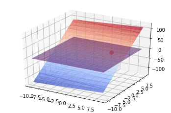
Example 5
Find the minimum value of following function. \(f(x) = 0.5x_1^2 + 5.5 x_2^2\)
Find numerical solution starting from $x_1 = 5, x_2 = 1 $
1
2
3
4
5
6
7
8
9
10
11
12
13
14
15
16
17
x1 = np.arange(-10, 10, 1)
x2 = np.arange(-10, 10, 1)
x1, x2 = np.meshgrid(x1, x2)  # outer product by ones_like(x1) or ones_like(x2)
# x1 = np.outer(np.linspace(-10, 10, 100), np.ones(100))
# x2 = x1.copy().T
y = 0.5*x1**2 + 5.5*x2**2
yprime = x1 + 11*x2
hyperplane = np.zeros_like(x1)
print(x1.shape, x2.shape, y.shape)

fig = plt.figure()
ax = plt.axes(projection='3d')
ax.plot_surface(x1, x2, yprime, cmap='coolwarm', alpha=0.7)
ax.contour(x1, x2, yprime, cmap='coolwarm', alpha=0.7)
ax.plot_surface(x1, x2, hyperplane, cmap='viridis', alpha=0.5)
ax.scatter([5], [1], [5 + 11 * 1], s=60 ,color='red')
plt.show()
1
2
(20, 20) (20, 20) (20, 20)
https://math.stackexchange.com/questions/3254520/computing-hessian-in-python-using-finite-differences
https://math.stackexchange.com/questions/2053229/the-connection-between-the-jacobian-hessian-and-the-gradient
Please note that the hessian matrix can be computed as transpose of the jacobian of gradient.
\(\mathbf{H}(f(x)) = \mathbf{J}(\nabla f(\mathbf{x}))^T\)
1
2
3
def f(x):
    """ x: shape=[2] """
    return 0.5*(x[0]**2) + 5.5*(x[1]**2)
1
gradient(f, [5, 1])
1
array([ 5., 11.])
1
2
3
4
5
6
7
8
9
10
11
12
13
14
15
16
17
18
19
20
def gradient(f, x, epsilon=1e-7):
    """ numerically find gradients.
    x: shape=[2] """
    grad = np.zeros_like(x, dtype=float)
    for i in range(len(x)):
        h = np.zeros_like(x, dtype=float)
        h[i] = epsilon
        grad[i] = (f(x + h) - f(x - h)) / (2 * h[i])
    return grad

def jacobian(f, m, x, epsilon=1e-10):
    """ numerically find gradients.
    f: shape=[m]
    x: shape=[n] """

    jaco = np.zeros(shape=(m, len(x)), dtype=float)
    for i in range(m):
        jaco[i, :] = gradient(lambda e: f(e)[i], x)

    return jaco
1
2
3
4
5
6
7
init = [5., 1.]
res = jacobian(lambda e: gradient(f, e), m=2, x=init) # this is hessian
print(res)
# therefore, hessian can be used as follows.
hessian = lambda f, m, x: jacobian(lambda e: gradient(f, e), m, x)

hessian(f, m=2, x=init)
1
2
3
[[ 0.976996  0.088818]
 [ 0.088818 11.10223 ]]
1
2
array([[ 0.976996,  0.088818],
       [ 0.088818, 11.10223 ]])
1
2
H_inv = np.linalg.inv(hessian(f, m=2, x=init))
H_inv
1
2
array([[ 1.02429 , -0.008194],
       [-0.008194,  0.090138]])
1
2
3
4
5
6
7
8
9
10
11
12
13
14
15
16
17
18
19
20
21
22
23
24
25
26
27
28
29
30
31
32
33
34
35
36
37
38
39
40
41
def newton(f, m, init, epsilon=1e-7, verbose=True, history=False):
    """ Newton Raphson Method.
    f: function
    m: the number of output dimension
    init: np.array, with dimension n """

    def gradient(f, x, epsilon=1e-7):
        """ numerically find gradients.
        x: shape=[2] """
        grad = np.zeros_like(x, dtype=float)
        for i in range(len(x)):
            h = np.zeros_like(x, dtype=float)
            h[i] = epsilon
            grad[i] = (f(x + h) - f(x - h)) / (2 * h[i])
        return grad

    def jacobian(f, m, x, epsilon=1e-10):
        """ numerically find gradients.
        f: shape=[m]
        x: shape=[n] """
        jaco = np.zeros(shape=(m, len(x)), dtype=float)
        for i in range(m):
            jaco[i, :] = gradient(lambda e: f(e)[i], x)

        return jaco

    hessian = lambda f, n, x: jacobian(lambda e: gradient(f, e), n, x)

    x = deepcopy(init)
    bound = 1e-7
    memo = [x]
    while True:
        H_inv = np.linalg.inv(hessian(f, n=len(x), x=x))
        update = np.matmul(H_inv, gradient(f, x))
        x = x - update
        if bound > sum(np.abs(update)):
            break
        if verbose: print("x={}, update={}".format(x, sum(np.abs(update))))
        if history: memo.append(x)
    if not history: return x
    return x, np.array(list(zip(*memo)))
1
2
3
4
ans, history = newton(f, m=1, init=np.array([5, 1], dtype=float), verbose=True, history=True)
print("history.shape={}".format(history.shape))
f(ans)
gradient(f, ans)
1
2
3
4
5
x=[-0.031314  0.049459], update=5.981855423871908
x=[-7.739249e-07  5.244940e-08], update=0.08077178497943122
x=[1.376429e-21 0.000000e+00], update=8.263742810599175e-07
history.shape=(2, 4)
1
array([0., 0.])
1
[f(vector) for vector in history.T]
1
[18.0, 0.013944122571079616, 3.1461002793436933e-13, 9.472777618835763e-43]
1
2
3
4
5
6
7
8
9
10
11
12
13
14
15
16
17
18
19
20
21
22
23
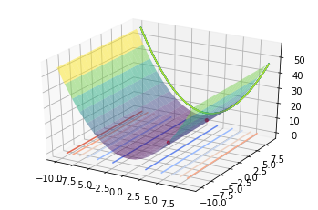
x1 = np.arange(-10, 10, 1)
x2 = np.arange(-10, 10, 1)
x1, x2 = np.meshgrid(x1, x2) # outer product by ones_like(x1) or ones_like(x2)
y = 0.5*x1**2 + 5
.5*x2**2
hyperplane = np.zeros_like(x1)
print(x1.shape, x2.shape, y.shape)
""" 3D figure """
fig = plt.figure()
ax = plt.axes(projection='3d')
ax.contour(x1, x2, y, cmap='coolwarm', zdir='z', offset=0, alpha=1)
ax.contour(x1, x2, y, zdir='y', offset=10, alpha=1)
ax.plot_surface(x1, x2, y, cmap='viridis', alpha=0.5)
ax.scatter(history[0, :], history[1, :], [f(vector) for vector in history.T], s=10 ,color='red')
""" 2D figure """
# ax = plt.axes()
# ax.contour(x1, x2, y, cmap='coolwarm', alpha=1)
# ax.scatter(history[0, :], history[1, :], s=5 ,color='red')
plt.grid(linestyle='--')
plt.show()
1
2
(20, 20) (20, 20) (20, 20)
Reference
[1] Dark Programmer’s blog - Newton method
[2] ” - gradient, jacobian, hessian, laplacian
[3] problems
Summary
제약사항:
- f(x)가 연속이고, 미분가능해야 한다.
- 해가 여러개인 경우 초기 값에 따라 수렴하는 해가 달라질 수 있다.
- 연립 방정식을 풀 경우, jacobian과 역행렬(만약 역행렬이 존재하지 않는 경우엔 pseudo inverse를 이용)을 구해야 한다.
- 만약 그 pseudo inverse가 singular 행렬(역행렬이 존재하지 않는 행렬)에 근접한 경우에는 계산된 역행렬이 수치적으로 불안정하여 해가 발산할 수 있는 문제점이 있다.
특징: 한번에 많은 이동을 하기 때문에 수렴이 빠를 수 있다. 하지만, 각각의 iteration 마다 jacobian과 역함수 혹은 hessian과 그 역함수를 구하는 것은 값비싼 연산이다. (Talyor Series를 이용해서 근사함으로서 구하는 방식도 사용 가능한 것 같다. 확실치 않아 좀더 공부해야할 것 같음)
추가적 내용
Newton Raphson Method 방식은 각 iteration마다 jacobian 혹은 hessian을 필요로 하는 경우까지 생길 수 있어, 그 matrix를 계산하는 것은 부담이 상당히 크다. 따라서 이 matrix를 근사하던지 좀더 변형된 방식으로 구하는 Gradient Descent, Quasi-Newton, BFGS, DFP 등이 있다. 나중에 다루어 보도록 하겠다.Memo: 정리할 내용
- gradient, jacobian, hessian, laplacian 계산 및 의미
- least square, pseudo inverse 관련 내용
- 다른 종유의 optimization 방식: 다음 포스팅은 gradient descent
- 테일러 급수에 대해

Leave a comment