Gradient Descent Algorithm on Python and Visualization

In [1]:

import numpy as np
from matplotlib import pyplot as plt
from copy import deepcopy
from mpl_toolkits import mplot3d

Gradient Descent Method

어떤 함수의 극소/극대 값을 구하기 위해 현재의 위치에서 변화율이 가장 큰 방향으로 이동하는 방식. 각 iteration마다 gradient를 구해야한다.

wikipedia의 example들에 대해 실험해볼 것이다.

Example 1

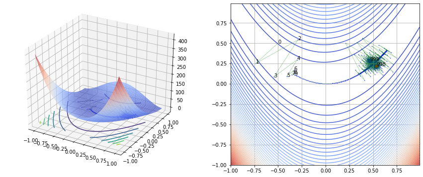
\[\begin{align} f(x_1, x_2) = (1 - x_1)^2 + 100(x_2 - x_1^2)^2 \\ \end{align}\]

In [2]:

x1 = np.arange(-1, 1, 0.01)
x2 = np.arange(-1, 1, 0.01)
print(x1.shape, x2.shape)
x1, x2 = np.meshgrid(x1, x2)  # outer product by ones_like(x1) or ones_like(x2) 

def f(x):
    f = (1 - x[0]) ** 2 + 100 * (x[1] - x[0] ** 2) **2
    return f

x = np.concatenate((x1[np.newaxis, :], x2[np.newaxis, :]), axis=0)
print(x[0].shape, x[1].shape)
y = np.array(f(x))
print(x1.shape, x2.shape, y.shape)

(200,) (200,)
(200, 200) (200, 200)
(200, 200) (200, 200) (200, 200)

Gradient Descent Recurrence

\(\mathbf{x}_{i + 1} = \mathbf{x}_i - \gamma \nabla f(\mathbf{x}_i)\)

In [3]:

def gradient(f, x, epsilon=1e-7):
    """ numerically find gradients. 
    x: shape=[n] """
    grad = np.zeros_like(x, dtype=float)
    for i in range(len(x)):
        h = np.zeros_like(x, dtype=float)
        h[i] = epsilon
        grad[i] = (f(x + h) - f(x - h)) / (2 * h[i])
    return grad

def jacobian(f, m, x, epsilon=1e-7, verbose=False):
    """ numerically find gradients, constraint: m > 1
    f: shape=[m]
    x: shape=[n] """
    jaco = np.zeros(shape=(m, len(x)), dtype=float)
    for i in range(m):
        jaco[i, :] = gradient(lambda e: f(e)[i], x)
    if m != len(x) or np.linalg.matrix_rank(jaco) != m: 
        if verbose: print('jacobian is singular, use pseudo-inverse')    
    return jaco

In [4]:

init = np.array([-0.5, 0.5])
print(f(init))
gradient(f, x=init)

8.5

array([46.99999998, 49.99999999])

Gradient Descent Implementation

In [5]:

def grad_decent(f, init, step, lr=0.001, history=False):
    x = deepcopy(init)
    memo = [x]
    for i in range(step):
        grad = gradient(f, x)
        x = x - lr * grad
        if history: memo.append(x)
    if not history: return x
    return x, np.array(list(zip(*memo)))

In [6]:

n_step = 1000
ans, history = grad_decent(f, init, step=n_step, lr=0.005, history=True)
print(ans)
print(history.shape)
f(ans)

[0.53552251 0.22117275]
(2, 1001)

0.6462276891526653

In [7]:

fig, (ax1, ax2) = plt.subplots(nrows=1, ncols=2, figsize=(15, 6))
ax1.remove()
ax1 = fig.add_subplot(1, 2, 1, projection='3d')
ax1.plot_surface(x1, x2, y, cmap='coolwarm', alpha=0.7)
ax1.contour(x1, x2, y, zdir='z', offset=0)
ax1.contour(x1, x2, y, zdir='y', offset=35)
ax1.scatter(history[0, :], history[1, :], [f(vec) for vec in history.T], s=2, color='blue', linewidth=0.5, alpha=0.5)
ax1.plot(history[0, :], history[1, :], [f(vec) for vec in history.T], color='black', linewidth=0.5, alpha=0.5)

ax2.contour(x1, x2, y, levels=50, cmap='coolwarm', alpha=1)
ax2.scatter(history[0, :], history[1, :], s=1, color='blue', alpha=0.5)
order = list(range(len(history[0])))
for i, txt in enumerate(order):
    if 0 <= i < 10 or (n_step - 3 < i < n_step):
        ax2.annotate(txt, (history[0][i], history[1][i]))
ax2.plot(history[0, :], history[1, :], color='green', linewidth=0.5, alpha=0.6)
ax2.scatter(ans[0], ans[1], s=30, color='red')
# ax2.set_xlim(-0.8, 0.8)
# ax2.set_ylim(-0.1, 1.1)
ax2.grid('--')

plt.show()

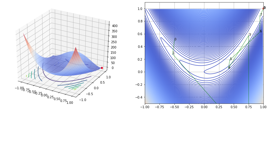
Gradient Desent vs Newton Raphson

Newton Rapshon 방법은 $f’ = 0$ 인 해를 찾아야한다.
이때, 매 iteration마다 hessian을 계산해야한다.
초기 값에 따라, 극소 점에 도달할 수도 극대점에 도달할 수도, 발산 할 수도 있다.

In [8]:

def newton(f, m, init, epsilon=1e-7, verbose=True, history=False, max_iter=1000):
    """ Newton Raphson Method.
    f: function 
    m: the number of output dimension
    init: np.array, with dimension n """
    hessian = lambda f, n, x: jacobian(lambda e: gradient(f, e), n, x)
    
    x = deepcopy(init)
    bound = 1e-7
    memo = [x]
    while max_iter:
        H_inv = np.linalg.inv(hessian(f, n=len(x), x=x))
        update = np.matmul(H_inv, gradient(f, x))
        x = x - update
        if bound > sum(np.abs(update)):
            break
        if verbose: print("x={}, update={}".format(x, sum(np.abs(update))))
        if history: memo.append(x)
        max_iter -= 1
    if not history: return x
    return x, np.array(list(zip(*memo)))

In [9]:

ans, history = newton(f, m=1, init=init, history=True, max_iter=100)
print(history.shape)
print(ans)
f(ans)

x=[-0.53070834  0.28068187], update=0.2500264708543467
x=[ 0.75125147 -1.07901222], update=2.641653901637466
x=[0.7507615  0.57230083], update=1.6518030179871521
x=[0.40914555 0.05069979], update=0.863216997087727
x=[0.4334482  0.18728728], update=0.16089013656989948
x=[0.93953274 0.62659491], update=0.9453921697257455
x=[0.94055255 0.88458658], update=0.2590114781322731
x=[0.99938126 0.99530208], update=0.16954421862361163
x=[0.99974724 0.99949442], update=0.004558318389770166
x=[0.99999999 0.99999992], update=0.0007582534925565458
(2, 11)
[1. 1.]

4.438902182203765e-24

In [10]:

fig, (ax1, ax2) = plt.subplots(nrows=1, ncols=2, figsize=(15, 6))
ax1.remove()
ax1 = fig.add_subplot(1, 2, 1, projection='3d')
ax1.plot_surface(x1, x2, y, cmap='coolwarm', alpha=0.7)
ax1.contour(x1, x2, y, zdir='z', offset=0)
ax1.contour(x1, x2, y, zdir='y', offset=10)
ax1.scatter(history[0, :], history[1, :], [f(vec) for vec in history.T], s=2, color='blue', linewidth=0.5, alpha=0.5)
ax1.plot(history[0, :], history[1, :], [f(vec) for vec in history.T], color='black', linewidth=0.5, alpha=0.5)
ax1.scatter(ans[0], ans[1], s=30, color='red')
# ax1.set_xlim(-1, 1)
# ax1.set_ylim(-1, 1)

ax2.contour(x1, x2, y, levels=500, cmap='coolwarm', alpha=1)
ax2.scatter(history[0, :], history[1, :], s=2, color='blue', alpha=0.5)
order = list(range(len(history[0])))
for i, txt in enumerate(order):
    if 0 <= i < 10 or (n_step - 3 < i < n_step):
        ax2.annotate(txt, (history[0][i], history[1][i]))
ax2.plot(history[0, :], history[1, :], color='green', linewidth=1, alpha=0.8)
ax2.scatter(ans[0], ans[1], s=30, color='red')
ax2.set_xlim(-1, 1)
ax2.set_ylim(-0.5, 1.1)
ax2.grid('--')

plt.show()

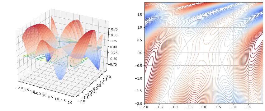
Example 2

\[\begin{align} f(x_1, x_2) = sin(\frac{1}{2}x_1^2 - \frac{1}{4}x_2^2 + 3) + cos(2x_1 + 1 - e^{x_2}) \end{align}\]

In [11]:

x1 = np.arange(-2, 2, 0.01)
x2 = np.arange(-2, 2, 0.01)
print(x1.shape, x2.shape)
x1, x2 = np.meshgrid(x1, x2)  # outer product by ones_like(x1) or ones_like(x2) 

def f(x):
    f = np.sin((x[0] ** 2) / 2 - (x[1] ** 2) / 4 + 3) * np.cos(2 * x[0] + 1 - np.exp(x[1]))
    return f

x = np.concatenate((x1[np.newaxis, :], x2[np.newaxis, :]), axis=0)
print(x[0].shape, x[1].shape)
y = np.array(f(x))
print(x1.shape, x2.shape, y.shape)

fig, (ax1, ax2) = plt.subplots(nrows=1, ncols=2, figsize=(15, 6))
ax1.remove()
ax1 = fig.add_subplot(1, 2, 1, projection='3d')
ax1.plot_surface(x1, x2, y, cmap='coolwarm', alpha=0.7)
ax1.contour(x1, x2, y, zdir='z', offset=0)

ax2.contour(x1, x2, y, levels=50, cmap='coolwarm', alpha=1)
# ax2.set_xlim(-0.8, 0.8)
# ax2.set_ylim(-0.1, 1.1)
ax2.grid('--')


plt.show()

(400,) (400,)
(400, 400) (400, 400)
(400, 400) (400, 400) (400, 400)

In [12]:

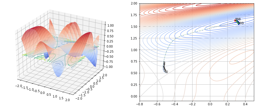
init = np.array([-0.5, 0.5])
print(f(init))

n_step = 1000
ans, history = grad_decent(f, init, step=n_step, lr=0.1, history=True)
print(ans)
print(history.shape)
f(ans)

-0.006150637545794505
[0.28554963 1.63180599]
(2, 1001)

-0.6387682772794055

In [13]:

fig, (ax1, ax2) = plt.subplots(nrows=1, ncols=2, figsize=(15, 6))
ax1.remove()
ax1 = fig.add_subplot(1, 2, 1, projection='3d')
ax1.plot_surface(x1, x2, y, cmap='coolwarm', alpha=0.7)
ax1.contour(x1, x2, y, zdir='z', offset=0)
ax1.scatter(history[0, :], history[1, :], [f(vec) for vec in history.T], s=2, color='blue', linewidth=0.5, alpha=0.5)
ax1.plot(history[0, :], history[1, :], [f(vec) for vec in history.T], color='black', linewidth=0.5, alpha=0.5)

ax2.contour(x1, x2, y, levels=50, cmap='coolwarm', alpha=1)
ax2.scatter(history[0, :], history[1, :], s=1, color='blue', alpha=0.5)
order = list(range(len(history[0])))
for i, txt in enumerate(order):
    if 0 <= i < 10 or (n_step - 3 < i < n_step):
        ax2.annotate(txt, (history[0][i], history[1][i]))
ax2.plot(history[0, :], history[1, :], color='green', linewidth=0.5, alpha=0.6)
ax2.scatter(ans[0], ans[1], s=30, color='red')
ax2.set_xlim(-0.8, 0.5)
ax2.set_ylim(-0.1, 2)
ax2.grid('--')

plt.show()

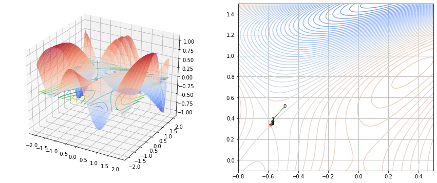
Newton Raphson 방법과 비교

In [14]:

ans, history = newton(f, m=1, init=init, history=True, max_iter=100)
print(history.shape)
print(ans)
f(ans)

x=[-0.57739683  0.37342925], update=0.20396758882610938
x=[-0.58304284  0.34137614], update=0.03769911383379125
x=[-0.58363898  0.33899018], update=0.0029820968988535186
x=[-0.5836422   0.33897761], update=1.5787065540124905e-05
(2, 5)
[-0.5836422   0.33897761]

-1.5518943484129243e-29

In [15]:

fig, (ax1, ax2) = plt.subplots(nrows=1, ncols=2, figsize=(15, 6))
ax1.remove()
ax1 = fig.add_subplot(1, 2, 1, projection='3d')
ax1.plot_surface(x1, x2, y, cmap='coolwarm', alpha=0.7)
ax1.contour(x1, x2, y, zdir='z', offset=0)
ax1.scatter(history[0, :], history[1, :], [f(vec) for vec in history.T], s=2, color='blue', linewidth=0.5, alpha=0.5)
ax1.plot(history[0, :], history[1, :], [f(vec) for vec in history.T], color='black', linewidth=0.5, alpha=0.5)
ax1.scatter(ans[0], ans[1], s=30, color='red')
# ax1.set_xlim(-1, 1)
# ax1.set_ylim(-1, 1)

ax2.contour(x1, x2, y, levels=100, cmap='coolwarm', alpha=1)
ax2.scatter(history[0, :], history[1, :], s=2, color='blue', alpha=0.5)
order = list(range(len(history[0])))
for i, txt in enumerate(order):
    if 0 <= i < 10 or (n_step - 3 < i < n_step):
        ax2.annotate(txt, (history[0][i], history[1][i]))
ax2.plot(history[0, :], history[1, :], color='green', linewidth=1, alpha=0.8)
ax2.scatter(ans[0], ans[1], s=30, color='red')
ax2.set_xlim(-0.8, 0.5)
ax2.set_ylim(-0.1, 1.5)
ax2.grid('--')

plt.show()

Example 3: Solution of a non-linear system

Gradient descent can also be used to solve a system of nonlinear equations.

objective function을 만들고, 이를 최소화하는 위치를 찾는다.

\[\begin{align} \begin{cases} 3x_1 - cos(x_2 x_3) - \frac{3}{2} = 0\\ 4x_1^2 - 625x_2^2 + 2x_2 - 1 = 0\\ exp(-x_1 x_2) + 20 x_3 + \frac{10 \pi - 3}{3} = 0\\ \end{cases} \end{align}\]

let $\mathbf{G}$ be as follows. \(G = \begin{bmatrix} 3x_1 - cos(x_2 x_3) - \frac{3}{2} \\ 4x_1^2 - 625x_2^2 + 2x_2 - 1 \\ exp(-x_1 x_2) + 20 x_3 + \frac{10 \pi - 3}{3} \\ \end{bmatrix}\)

$\mathbf{F} = \frac{G^T G}{2}$ 로 두고, F의 최솟값이 되는 $\mathbf{x}$ 위치를 찾는다.

Recall that

\[\mathbf{x}_{i + 1} = \mathbf{x}_i - \gamma \nabla F(\mathbf{x}_i)\]

In [16]:

init = [0, 0, 0]  # inital state
def G(x):
    g1 = 3 * x[0] - np.cos(x[1] * x[2]) - 3 / 2
    g2 = 4 * (x[0] ** 2) - 625 * (x[1] ** 2) + 2 * x[1] - 1
    g3 = np.exp(-x[0] * x[1]) + 20 * x[2] + (10 * np.pi - 3) / 3
    return np.array([g1, g2, g3])

def F(x):
    """ x: np.array, shape=[3] """
    return np.dot(G(x).T, G(x)) / 2

print(G(init))
print(F(init))
gradient(F, x=init)

[-2.5        -1.         10.47197551]
58.45613556160755

array([ -7.50000002,  -1.99999999, 209.43951029])

In [17]:

n_step = 1000
ans, history = grad_decent(F, init, step=n_step, lr=0.001, history=True)
print(ans)
print(history.shape)
F(ans)

[ 0.73056362  0.02538866 -0.5220892 ]
(3, 1001)

0.35396182672082166

활용: ML 모델 파라미터 결정 관점

주어진 데이터 ($\mathbf{x}, \mathbf{y}$)가 있을때 모델 $f_{\theta}(\mathbf{x})$ 를 통해 $y$를 예측. $\theta$(모델의 파라미터)를 어떻게 결정 할까?

• 여러 방법이 존재. 그 중 가장 간단한 방법 중 하나인 gradient decent 방식에 대해 알아보았다. (다음에는 업데이트로 찾는게 아니라 바로 해를 찾는 least square에 대해 알아볼 예정)

gradient descent vs stocastic gradient descent

gradient descent은 ML(Mechine Learning)에서 사용가능. 모델의 예측 과 실제 값 사이의 오차를 줄이도록, 모델의 파라미터 값 결정. 모델의 파라미터를 업데이트할 기울기를 구하는데 크게 2가지 방식으로 나뉨.

1. 전체 데이터에 대한 기울기를 구하는 (steepest) gradient descent 방식
2. 미니 배치의 기울기를 구하는 stochastic gradient descent 방식.

Reference

[1] gradient descent - wiki
[2] korean blog

Future

optimization 계보를 바탕으로 학습하겠다.

Summary

1. Gradient Descent :
   • step size가 필요하다. 이로 인해 수렴할 때 속도차이가 생긴다.
2. Newton Raphson
   • $f’(x) = 0$ 인 x를 구하기 때문에 극대/극소를 구분할 수가 없다. 이를 구분하기 위해 Hessian 테스트라는 것을 이용해야 한다.