Rejection Sampling

Rejection Sampling

내용 이해

곧바로 샘플링 하기 힘든 분포에서 샘플을 뽑기 위한 방법.

샘플링 하고 싶은 분포는 타겟 분포 $p(x)$라 하자.

**타겟분포 $p(x)$에 대한 샘플 $X = {x}_{i=1, 2, \cdots, N}$을 얻고자할때 샘플링 하기 쉬운 분포 $q(x)$ 를 이용하는 trick**이다.

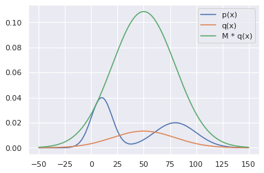
$q(x)$의 필요 조건은 다음식을 만족하는 $M$을 파라미터로 두어야한다(1보다 큰 값). \(Mq(x) \ge p(x)\)

다음 그림을 보면 이해하기 쉽다.

즉, $q$ 에서 샘플을 생성하여 $[0, Mq(x_0)]$ 사이의 난수에 따라 샘플을 기각-수용하는 과정을 무한히 반복하면, rejection sampling을 통해 얻은 샘플들은 결국 다음과 같이 $p$에서 생성된 샘플처럼 보이게 된다.

pseudo code는 다음과 같다.

https://untitledtblog.tistory.com/134

https://wiseodd.github.io/techblog/2015/10/21/rejection-sampling/

구현

In [6]:

import numpy as np
import scipy.stats as st  # statistics 관련된 라이브러리
import seaborn as sns  # 확률 분포 관련 라이브러리
import matplotlib.pyplot as plt

In [7]:

sns.set()

In [8]:

class Distribution:
    
    def __init__(self, q_mu=50, q_std=30):
        """ I merge two normal distributions in order to build complex distribution. 
        `loc`: mean
        `scale`: standard deviation
        """
        
        # target distribution, that is, complex distribution. 
        # assume that we do not know loc and scale.
        self.p = lambda x: st.norm.pdf(x, loc=10, scale=10) + \
                            st.norm.pdf(x, loc=80, scale=20)  
        
        # known distribution, sampling from this distribution.
        self.q = lambda x: st.norm.pdf(x, loc=q_mu, scale=q_std)        
        self.q_mu = q_mu
        self.q_std = q_std

In [9]:

ds = Distribution()
x = np.arange(-50, 151)  # 범위 지정
M = max(ds.p(x) / ds.q(x))  # M 설정; 1에 가까울수록 좋음. 
M

8.158929050400344

In [10]:

fig, ax = plt.subplots()
print(fig, ax)
ax.plot(x, ds.p(x), label='p(x)')
ax.plot(x, ds.q(x), label='q(x)')
ax.plot(x, M * ds.q(x), label='M * q(x)')
ax.legend()
fig.show()

Figure(432x288) AxesSubplot(0.125,0.125;0.775x0.755)

<ipython-input-10-f7031b52d24b>:7: UserWarning: Matplotlib is currently using module://ipykernel.pylab.backend_inline, which is a non-GUI backend, so cannot show the figure.
  fig.show()

샘플링을 해보자.

In [21]:

def rejection_sampling(N, M, ds:Distribution):
    samples = []  
    n = 0
    while n < N:
        x0 = np.random.normal(ds.q_mu, ds.q_std)  # a sample from known(easy) distribution.
        u = np.random.uniform(0, M*ds.q(x0))  # uniform sample in [0, M*q(x0)]

        if u <= ds.p(x0):  # accept
            samples.append(x0) 
            n += 1
        else: None # reject 
            
    return np.array(samples)

In [22]:

samples = rejection_sampling(N=10000, M=M, ds=ds)

In [23]:

samples.shape

(10000,)

다루기쉬운 uniform 분포로부터 원하는 분포를 가진 샘플을 얻었다. 비록 타겟분포가 뭔지는 모르지만 충분한 샘플들을 얻었다는 것이 rejection sampling을 하는 이유이다.

In [25]:

sns.distplot(samples)

<matplotlib.axes._subplots.AxesSubplot at 0x7f3ecf8c9d00>

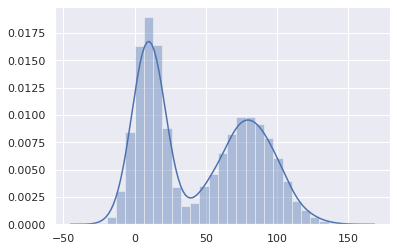
샘플들에 대한 mean과 std를 출력해보면 다음과 같다.

In [32]:

print(f"mean of samples: {np.mean(samples)}")
print(f"std of samples: {np.std(samples)}")

mean of samples: 45.0493101546719
std of samples: 38.26204218755405

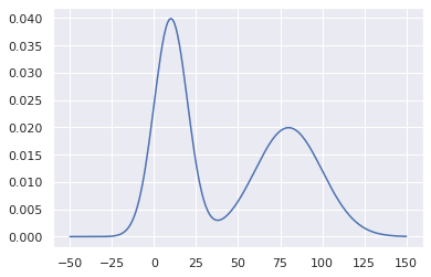
아래는 실제로 얻기 힘든 $p(x)$를 출력해보았다. 위의 샘플들에 의한 결과에 상당히 비슷한 경향을 보임을 알 수 있다.

In [33]:

fig, ax = plt.subplots()
print(fig, ax)
ax.plot(x, ds.p(x), label='p(x)')

Figure(432x288) AxesSubplot(0.125,0.125;0.775x0.755)

[<matplotlib.lines.Line2D at 0x7f3ece17a040>]

활용

LinUSB1 논문에서 policy evalution을 위한 샘플 데이터 취득을 rejection sampling을 이용한다.

환경(실생활)과 상호작용(강화학습)을 통해 어떤 원하는 타겟 분포를 예측하고, 보상을 최대화 하는 행동을 예측하는 것이 중요한 문제이다.

위의 논문에서 확률 분포를 예측해도 실생활에서의 확률 분포를 알아낼 수는 없기 떄문에 그 예측이 잘 맞아 떨어지는지 확인하기가 어렵다. 따라서, rejected sampling 을 통해 실제 확률분포와 가장 유사한 테스트 샘픔들을 모아놓고, 그 테스트 샘플을 통한 행동 예측에 따라 평균 보상 값을 구하면 합당한 평가 기준이 될 수 있다고 본다.