Ristricted Boltzmann Machine

In [1]:

%load_ext autoreload
%autoreload 2

In [2]:

from jupyterthemes import jtplot
jtplot.style(theme='monokai', context='notebook', ticks=True, grid=False)

Boltzman Machine

분자운동을 모델링한 결과 관계있는 것들은 같이 움직이는 것을 포착하는 경향을 보였다는 아이디어로부터 입력 패턴을 clustering하는 노드들을 찾는 방법이다.

geeksforgeeks 의 이 article¹ 에 따르면 볼츠만 머신은 다음과 같은 성향을 띄는 모델이라고 정리하였다.

Boltzmann Machines is an unsupervised DL model in which every node is connected to every other node.
Boltzmann Machine is not a deterministic DL model but a stochastic or generative DL model.

즉, 볼츠만 머신은 입력만 가지고 그 입력에 대한 representation을 찾아주는 모델이다.

---

[1]: Types of Boltzman Machines

Energy Based Model

분자들의 운동을 모델링 했다는 것은 무엇일까? 분자들의 움직임을 설명하는 분포는 에너지의 총량이 일정한 상태에서 엔트로피를 최대화하는 형태이다. 이것을 수학적으로 문제를 정의하면 다음과 같다.

엔트로피를 최대화하는 분포 $p(x)$를 찾고자 함. 이 때 $x$는 분자의 state이며 에너지 총량은 $\alpha$.

\[\begin{align} \underset{p(x)}{max}\;-\sum_{x}&{p(x)\ln p(x)} \;\; s.t. \; \sum_{x}p(x) = 1, \alpha = \sum_{x}p(x)E(x) \end{align}\]

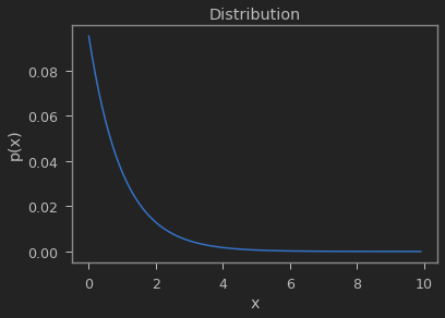
위의 최적화 문제의 해의 형태는 다음과 같으며 이러한 해의 분포를 Boltzman 분포라고 한다.

(여기서 $Z$ 는 $\sum_{x}p(x) = 1$ 을 만족하도록 하는 partition function 인 $Z = \sum_{x}{e^{-E(x)}}$ 이다.)

\[\begin{align} p(x) = \frac{e^{-E(x)}}{Z} \\ \end{align}\]

이 분포는 결국 Energe $E(x)$를 찾는 것이 관건이다. $E(x)$ 를 찾는 모델은 Energy based Model 이라 불리운다.

In [3]:

import numpy as np
import matplotlib.pyplot as plt

def p(x):
    y = np.exp(-x)
    Z = np.sum(y)
    return y / Z

x = np.arange(0, 10, 0.1)
plt.plot(x, p(x))
plt.xlabel("x")
plt.ylabel("p(x)")
plt.title("Distribution")

Text(0.5, 1.0, 'Distribution')

Boltzman Energy Function

Boltzman Machine에서는 Energy function을 다음과 같이 모델링한다.

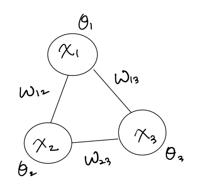
여기서 유닛 사이의 weight 는 $W$ 각 유닛의 에너지 함수에 대한 bias 는 $\theta$이다.

대부분 $W$ 는 symmetric matrix 이며 대각 성분은 $0$이다.

\[\begin{align} E(x) &= -\frac{1}{2}x^{T}Wx - \theta^{T}x \\ &= -\underbrace{\sum_{k<j}x_{k}w_{kj}x_{j}}_{\text{weight term}} - \underbrace{\sum_{k}\theta_{k}x_{k}}_{\text{bias term}} \end{align}\]

Structure

구조는 그림처럼 hidden node와 visible node 가 fully connected로 구성되어 있으며 node사이의 관계는 $x^{t+1} = \sigma(W x^{t})$로 다음과 같다.

각 노드는 binary state 를 갖고 0과 1사이의 확률에 대한 임계값에 따라서 On/Off로 firing 된다.

Learning은 노드사이의 관계를 나타내는 weight $W$과 bias $\theta$를 찾는 것이고, Inference는 visible node들에 입력 패턴이 주어졌을 때 firing 되는 hidden node를 찾는 것이다.

Gibbs Sampling

볼츠만 머신은 각 노드의 분포를 어떻게 학습하는 걸까? Baysian inference 개념을 바탕으로 깁스 샘플링을 이용한다.

Boltzman Machine을 Gibbs Sampling²으로 Bayesian Inference 하는 과정에서는 다음과 같이 $i$ 번째 노드의 값을 모르는 상태에서 $i$번째 노드가 firing할 확률을 구한다. ($-i$ 는 $i$ 인덱스 제외한 나머지) \(\begin{align} \require{cancel} p(x_{i}=1|x_{-i}) &= \frac{p(x_{i}=1, x_{-i})}{p(x_{i}=1, x_{-i}) + p(x_{i}=0, x_{-i})} \\ &= \frac{e^{-E(x_{i}=1, x_{-i})} }{ e^{-E(x_{i}=1, x_{-i})} + e^{-E(x_{i}=0, x_{-i})}} \\ &= \frac{1 }{ 1 + e^{-E(x_{i}=0, x_{-i}) + E(x_{i}=1, x_{-i}) }} \\ &= \frac{1 }{ 1 + e^{ \cancel{\sum_{k<j, k \neq i} x_{k}w_{kj}x_{j}} + \cancel{\sum_{k \neq i}\theta_{k}x_{k}} - \cancel{\sum_{k<j, k \neq i}x_{k}w_{kj}x_{j}} - \cancel{\sum_{k \neq i}\theta_{k}x_{k}} - \sum_{j \neq i}w_{ij}x_{j} - \theta_{i} } } \\ &= \frac{1 }{ 1 + e^{- \sum_{j \neq i}w_{ij}x_{j} - \theta_{i} } } \\ &= \sigma(\sum_{j \neq i}w_{ij}x_{j} + \theta_{i}) \end{align}\) 결과는 $i$번째 노드를 제외한 모든 노드들의 피드백을 더한 것을 의미한다.

---

[2]: mcmc.ipynb “MCMC and Gibbs Sampling”

Restricted Boltzman Machine

Boltzman Machine 은 모든 뉴런이 fully connected 되어있다. 그렇게 되면 학습해야 되는 리소스들이 많아져서 overhead가 증가한다. 필요 없는 연결은 제거해도 되지 않을까? 라는 motivation에서 Restricted Boltzman Machine, RBM 이 제안되었다.

RBM 은 다음과 같이 입력 노드와 히든 노드들에 의해 두 층으로 이루어지며 같은 layer의 노드끼리는 연결이 제한되어 있는 Unsupervised Learning문제를 푸는 확률론적인 모델이다. 신경망 구조의 시초라고 볼 수 있다.

모든 연결이 필요하지 않은 이유는 다음과 같다.

visible 노드는 입력 패턴에 의해서 이미 값이 결정되기 때문에 노드별 관계를 학습할 필요가 없다. 그리고 hidden 노드는 서로 독립적인 의미를 지니기 때문에 관계를 학습할 필요가 없다.

Training

RBM을 훈련시킬 때에는 두 개 이상의 확률변수의 결합확률분포로부터 일련의 표본을 생성하는 확률적 알고리즘인 Gibbs Sampling을 통해 훈련을 시킨다.

$h = \sigma(v^T W)$ 와 $v = \sigma(W^{T} h)$ 의 관계로 visible노드와 hidden 노드의 값을 구할 수 있다. 그렇게 하면 hidden node를 통해서 unsupervised learning 을 할 수 있다.

즉, RBM의 Energy 함수는 다음과 같으며 visible 노드와 hidden 노드간 correlation을 강화하는 방향으로 학습한다.

\[\begin{align} E(v,h) &= -v^{T}Wh - v^{T}b^{v} - h^{T}b^{h} \\ &= -\sum_{\forall i, j} v_{i}w_{i,j}h_{j} - \sum_{i} b^{v}_{i}v_{i} - \sum_{j} b^{h}_{j}h_{j} \\ & where \; v, b^{v} \in \mathbb{R}^{I}, \;\; h,b^{h} \in \mathbb{R}^{J}, \;\; W \in \mathbb{R}^{I \times J} \end{align}\]

위에서 visible 노드와 hidden노드간의 energy 함수 $E(v,h)$를 모델링 해보았다.

이번엔 우리가 관측하여 얻을 수 있는 likelihood 인 visible node의 확률 $p(v)$ 를 $E(v,h)$로 표현하여 likelihood를 최대화하는 $E(v,h)$ 의 파라미터를 학습하면 된다.

likelihood 는 $p(v \mid W, \theta)$ 인데 모델 파라미터에 관한 부분은 표기를 쉽게하기 위해 생략.

$E(v,h)$ 대한 energy based model인 Boltzman 분포 $p(v,h)$값을 구할수 있다. 그러면 hidden노드에 대한 값을 다음과 같이 marginalize 함으로써 $p(v)$를 구할 수 있다.

\[p(v) = \sum_{h} p(h) p(v|h) = \sum_{h} p(v,h) = \frac{\sum_{h} e^{-E(v,h)}}{Z} = \frac{e^{-F(v)}}{Z}\]

다시 visible node의 firing 확률분포 $p(v)$를 energy function $F(v)$에 대한 energy based model로 놓고 $F(v)$를 구하면 다음과 같다.

\[F(v) = - \ln \sum_{h} e^{-E(v,h)}\]

$p(v)$를 최대화한다는 것은 $F(v)$를 최소화하는 것과 같다. 최종적으로 RBM의 학습은 위와같은 logsumexp 함수를 최소화하는 $E(v,h)$의 파라미터를 찾으면 되는 것이다.

Stochastic Gradient Ascent

Stochastic Gradient Acent를 적용하여 weight가 어떻게 변화하는지 분석해보자.
logliklihood $\ln p(v)$ 를 stochastic gradient acent를 통해 학습하면 다음과 같다.
\(w_{ij} \leftarrow w_{ij} + \alpha \frac{\partial \ln p(v)}{ \partial w_{ij}} \vert_{v=v^{0}}\)

이어서 loglikelihood의 gradient를 계산해보자.

\[\begin{align} \frac{\partial \ln p(v)}{ \partial w_{ij}} \vert_{v=v^{0}} = -\underbrace{\frac{\partial F(v)}{ \partial w_{ij}} \vert_{v=v^{0}}}_{\text{Energy term}} -\underbrace{\frac{\partial \ln Z}{\partial w_{ij}}}_{\text{Partition term}} \end{align}\]

에너지 함수 부분과 분배함수 부분으로 나뉜다. 두 부분을 하나씩 유도해보자.
식의 간략화를 위해서 에너지 함수의 bias $b^{v}, b^{h} = 0$ 으로 가정한다.
우선 에너지 함수부분은 다음과 같다.

\[\begin{align} \frac{\partial F(v)}{ \partial w_{ij}} &= -\frac{\partial}{\partial w_{ij}} \ln \sum_{h} e^{-E(v,h)} \\ &= -\frac{\sum_{h} e^{-E(v,h)} (- \frac{\partial E(v,h)}{\partial w_{ij}})}{\sum_{h} e^{-E(v,h)}} \\ &= -v_{i}h_{j} \end{align}\]

따라서 $-\frac{\partial F(v)}{ \partial w_{ij}} \vert_{v=v^{0}} = v^{0}h_{j}$ 가 된다.

분배함수 부분은 다음 같다.

\[\begin{align} \frac{\partial \ln Z}{\partial w_{ij}} &= \frac{\partial}{\partial w_{ij}} \ln \sum_{v} e^{-F(v)} \\ &= \frac{1}{\sum_{v} e^{-F(v)}} \sum_{v} e^{-F(v)} \underbrace{(- \frac{\partial F(v)}{ \partial w_{ij}})}_{\text{ v에 종속적이라 소거 안됨}} \\ &= \frac{1}{Z} \sum_{v} e^{-F(v)} v_{i}h_{j} = \sum_{v} \frac{e^{-F(v)}}{Z} v_{i}h_{j} = \sum_{v} p(v) v_{i}h_{j} \\ &= \mathbb{E}_{p(v)} [v_{i}h_{j}] \end{align}\]

최종적으로 stochastic gradient acent로 weight변화량을 구하면 다음과 같다.

\[\Delta w_{ij} = \frac{\partial \ln p(v)}{ \partial w_{ij}} \vert_{v=v^{0}} = \underbrace{v_{i}^{0}h_{j}}_{data} - \underbrace{\mathbb{E}_{p(v)} [v_{i}h_{j}]}_{model}\]

의미적으로 보면 첫째항은 데이타 통계로부터 구한 visible 노드와 hidden노드의 correlation이고, 둘째항은 model 로부터 구한 visible 노드와 hidden노드의 correlation이다.

따라서 데이터와 모델의 visible 노드와 hidden노드 사이의 correlation에 대한 residual 만큼 weight를 업데이트 한다.

위의 식에서 두번째 항을 구하는데 문제가 발생한다.

$p(v) = \sum_{h} p(v,h)$ 인데, 결합 확률 분포 $p(v,h)$를 구하는게 일반적으로 어렵기 때문에(computation cost가 너무 크거나 혹은 구할 수 없는 경우) $\mathbb{E}_{p(v)}[v_i h_j]$를 계산할 수 없다.

이 경우 MCMC 방법으로 추정 할 수 있다. 특히 MCMC 방법중 Gibbs Sampling방법을 사용한다.

위에서 유도한 뉴런의 firing 확률 $p(x_{i}=1 \mid x_{-i}) = \sigma(\sum_{j \neq i}w_{ij}x_{j} + \theta_{i})$를 RBM에 적용하면 hidden 뉴런과 visible 뉴런의 firing 확률을 구할 수 있다.

$v^{0}, h^{0}$ 값을 임의로 설정하고 아래의 식을 따라 $v_{i}, h_{j}$가 수렴할 때 까지 반복하면 $\mathbb{E}_{p(v)}[v_i h_j]$ 값을 얻을 수 있다.

\[\begin{align} h_{j} \sim \sigma(w_{j}^Tv + \theta_{j}) \\ v_{i} \sim \sigma(w_{i}^{T}h + \theta_{i}) \end{align}\]

RBM의 학습은 깁스 샘플링을 통해 수행된다.

초기 모델에서 입력 데이터로 숨겨진 유닛들의 값들을 계산하고, 그 숨겨진 유닛들의 값들에서 다시 새로운 유닛들의 값들을 발생시킨다.

이 과정을 다음과 같이 무한 번 반복하면 초기 지점을 잊은 안정된 분포에서 샘플링을 할 수 있게 된다.

그러나 이 방법은 연산 양이 많은 문제가 있다.

이 과정을 유한 번 반복으로 비슷하게 구현할 수 있는 방법으로 대조적 발산 Contrastive Divergence, CD 이 있다.

Contrast Divergence

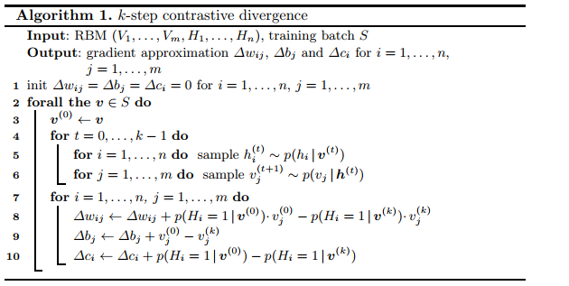
Contrastive Divergence 알고리즘을 한 마디로 요약하면 MCMC (Gibbs Sampling)의 step을 converge할 때 까지 돌리는 것이 아니라, 일정 수 만큼만 돌려서 approximate하고, 그 값을 사용하여 gradient의 업데이트에 사용하는 방법이다.

“어차피 정확하게 converge한 distribution이나, 중간에 멈춘 distribution이나 대략의 방향성은 공유할 것이다. 그렇기 때문에 완벽한 gradient 대신 Gibbs sampling을 중간에 멈추고 그 approximation 값을 update에 사용하자.” 라는 아이디어이다.

즉 $v_{i}, h_{j}$에 대해 $k$ step 동안 샘플링을 통해 $v_{i}^{0}, h_{j}^{0} \rightarrow \cdots \rightarrow v_{i}^{k}, h_{j}^{k}$를 반복한다.

모델을 학습하는 초기에는 모델이 정확하지 않아서 위의 반복이 무의미한 반복일 수 있다.

그래서 다음과 같이 gradient를 정의한다.

\[\frac{\partial \ln p(v)}{ \partial w_{ij}} \vert_{v=v^{0}} = v_{i}^{0}h_{j}^{0} - \underbrace{v_{i}^{k}h_{j}^{k}}_{CD-k}\]

위에서 정의한 gradient를 바탕으로 weight를 업데이트하면 효과적으로 학습을 할 수 있다.

알고리즘은 다음과 같다. (CD with $k$ steps of Gibbs Sampling)

여기서 주목할 점은 한번 업데이트 마다 Contrastive divergence 가 $k$번 수행되는데 distribution 에서 샘플링된다.

Contrastive Divergence 방법은 Hinton이 처음 제안한 이후 충분한 시간이 흐른 후에 전체 log likelihood의 local optimum으로 converge한다는 이론적 결과까지 증명된다.

An Application of RBM

kaggle 에 이 article의 코드를 바탕으로 구현. 음악에서 artist를 추천하는 것에 대한 내용이니 읽어 보면 좋을 듯 함.

사용된 데이터 셋은 다음과 같다. (Two dataset files were selected and preprocessed for use in this work)

• lastfm_user_scrobbles.csv contains $92,792$ scrobble counts (scrobbles) for $17,493$ artists (artist_id) generated by $1,892$ users (user_id).
• lastfm_artist_list.csv contains the list of $17,493$ artists, referenced by an unique id code (artist_id), the same used in the first file.

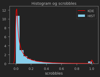
다음과 같은 이유로 위의 scrobble을 $0$ 과 $1$ 사이로 normalization하여 사용.

• Both heavy users, who have generated dozens, even hundreds of thousands of ‘scrobbles’ for selected artists, and light users, who produced few ‘scrobbles’ for few artists. The model must ideally not allow that heavy user preferences overshadow those of light users;
• For every user, the number of scrobbles per artist may vary from one to thousands. The model shall ideally not allow high scrobble counts per user to drastically overshadow low scrobble counts per user.

In [4]:

import warnings
from datetime import datetime

import numpy as np
import pandas as pd
import seaborn as sns
import torch

warnings.filterwarnings('ignore')
start_time = datetime.now()
print("starting date:", start_time)

scrobbles = pd.read_csv('./data/lastfm-music-artist-scrobbles/lastfm_user_scrobbles.csv', header = 0)
scrobbles['scrobbles'] = scrobbles.groupby('user_id')[['scrobbles']].apply(lambda x: (x-x.min())/(x.max()-x.min()))
scrobbles['scrobbles'] = scrobbles['scrobbles'].fillna(0.5)

print(scrobbles.shape)
scrobbles.head(3)

starting date: 2021-01-02 00:53:24.092904
(92792, 3)

	user_id	artist_id	scrobbles
0	1	4562	1.000000
1	1	10191	0.825509
2	1	494	0.798536

In [5]:

# 아래 링크는 distplot 사용 document.
# https://seaborn.pydata.org/tutorial/distributions.html
config = {"rug_kws": {"color": "green"}, 
          "kde_kws": {"color": "red", "linewidth": 2, "label": "KDE"}, 
          "hist_kws": {"linewidth": 5, "alpha": 1, "color": "skyblue", "label": "HIST"}}
sns.distplot(scrobbles['scrobbles'], kde=True, rug=False, bins=20, **config).set_title("Histogram og scrobbles")
# sns.pairplot(scrobbles)

Text(0.5, 1.0, 'Histogram og scrobbles')

The scrobbles dataset is originally sorted based on ascending user ids. As generating recommendations for specific users is the ultimate objective of this exercise, it is necessary to maintain user scrobbles grouped. In addition, as roughly $20%$ of user scrobbles will be segregated in a test set:

The training set will include the first $74,254$ scrobbles, corresponding to users with ‘user_id’ ranging from $1$ to $1,514$;

The test set will include the remaining $18,538$ scrobbles, corresponding to users with ‘user_id’ ranging from $1,515$ to $1,892$.

training set과 test set을 모델에서 쉽게 학습, 추론 단계에서 사용하기 위해 convert함수로 sparse한 matrix 꼴로 바꾸어 사용할 것이다.

In [6]:

def convert(f_data, f_nr_observations, f_nr_entities):
    """
    Generates (from a numpy array) a list of lists containing the number of hits per user (rows), per entity (columns).
    Each of the constituent lists will correspond to an observation / user (row).
    Each observation list will contain the number of hits (columns), one for each hit entity
    f_data - Input table (numpy array)
    f_nr_observations - Number of observations
    f_nr_entities - Number of entities hit in each observation
    """
    f_converted_data = []
    for f_id_user in range(1, f_nr_observations + 1):
        f_id_entity = f_data[:,1][f_data[:,0] == f_id_user].astype(int)
        f_id_hits = f_data[:,2][f_data[:,0] == f_id_user]
        f_hits = np.zeros(f_nr_entities)
        f_hits[f_id_entity - 1] = f_id_hits
        f_converted_data.append(list(f_hits))
    return f_converted_data

In [7]:

training_size = 74254
training_set = scrobbles.iloc[:training_size, :]  # Until userID = 1514
test_set = scrobbles.iloc[training_size:, :]      # Starting at userID = 1515

training_set = training_set.values
test_set = test_set.values

nr_users = int(max(max(training_set[:,0]), max(test_set[:,0])))
nr_artists = int(max(max(training_set[:,1]), max(test_set[:,1])))

training_set = convert(training_set, nr_users, nr_artists)
test_set = convert(test_set, nr_users, nr_artists)

training_set = torch.FloatTensor(training_set)
test_set = torch.FloatTensor(test_set)

print("the number of user and artist: ({}, {})".format(nr_users, nr_artists))
print("train-test information:", training_set.shape, test_set.shape)

the number of user and artist: (1892, 17493)
train-test information: torch.Size([1892, 17493]) torch.Size([1892, 17493])

In [8]:

def density_rate(sparse_matrix: torch.Tensor):
    return len(sparse_matrix.nonzero()) / (sparse_matrix.shape[0] * sparse_matrix.shape[1]) * 100

"density rate [%] - train: {0:0.4f}, test: {1:0.4f}".format(density_rate(training_set), density_rate(test_set))

'density rate [%] - train: 0.2160, test: 0.0540'

RBM Implementation

go to see rmb.py.

In [9]:

%%writefile rbm.py
import warnings
from datetime import datetime

import numpy as np
import pandas as pd
import torch

from verbose import printProgressBar

np.set_printoptions(precision=2, suppress=True)
torch.set_printoptions(precision=4, sci_mode=False)

print(f"torch version: {torch.__version__}")

class RestrictedBoltzmannMachine():
    """
    Python implementation of a Restricted Boltzmann Machine (RBM) with 'c_nh' hidden nodes and 'c_nv' visible nodes.
    """
    def __init__(self, c_nv, c_nh):
        """
        RBM initialization module where three tensors are defined:
        W - Weight tensor
        a - Visible node bias tensor
        b - Hidden node bias tensor
        a and b are created as two-dimensional tensors to accommodate batches of observations over training.
        """
        self.W = torch.randn(c_nh, c_nv)
        self.a = torch.randn(1, c_nh) 
        self.b = torch.randn(1, c_nv)
        
    def sample_h(self, c_vx):
        """
        Method devoted to Gibbs sampling probabilities of hidden nodes given visible nodes - p (h|v)
        c_vx - Input visible node tensor
        """
        c_w_vx = torch.mm(c_vx, self.W.t())
        c_activation = c_w_vx + self.a.expand_as(c_w_vx) # broadcast
        c_p_h_given_v = torch.sigmoid(c_activation)
        return c_p_h_given_v, torch.bernoulli(c_p_h_given_v) # probabilty, state

    
    def sample_v(self, c_hx):
        """
        Method devoted to Gibbs sampling probabilities of visible nodes given hidden nodes - p (v|h)
        c_hx - Input hidden node tensor
        """
        c_w_hx = torch.mm(c_hx, self.W)
        c_activation = c_w_hx + self.b.expand_as(c_w_hx)
        c_p_v_given_h = torch.sigmoid(c_activation)
        return c_p_v_given_h, torch.bernoulli(c_p_v_given_h)

    
    def train(self, c_nr_observations, c_nr_epoch, c_batch_size, c_train_tensor, c_metric, lr):
        """
        Method through which contrastive divergence-based training is performed.
        c_nr_observations - Number of observations used for training
        c_nr_epoch - Number of training epochs
        c_batch_size - Batch size
        c_train_tensor - Tensor containing training observations
        c_metric - Training performance metric of choice ('MAbsE' for Mean Absolute Error, 'RMSE' for Root Mean Square Error)
        """
        print('Training...')
        for c_epoch in range(1, c_nr_epoch + 1):
            c_start_time = datetime.now()
            c_train_loss = 0
            c_s = 0.
            for c_id_user in range(0, c_nr_observations - c_batch_size, c_batch_size):
                c_v0 = c_train_tensor[c_id_user:c_id_user+c_batch_size]  # c_batch_size x c_nv
                c_vk = c_train_tensor[c_id_user:c_id_user+c_batch_size]  # c_batch_size x c_nh
                c_ph0,_ = self.sample_h(c_v0)
                for c_k in range(10):
                    _,c_hk = self.sample_h(c_vk)
                    _,c_vk = self.sample_v(c_hk)
                    c_vk[c_v0<0] = c_v0[c_v0<0]
                c_phk,_ = self.sample_h(c_vk)
                self.W += lr*(torch.mm(c_v0.t(), c_ph0) - torch.mm(c_vk.t(), c_phk)).t()  # weight update
                self.b += lr*torch.sum((c_v0 - c_vk), 0)  # visible bias update
                self.a += lr*torch.sum((c_ph0 - c_phk), 0)  # hidden bias update
                if c_metric == 'MAbsE':
                    c_train_loss += torch.mean(torch.abs(c_v0[c_v0>=0] - c_vk[c_v0>=0]))
                elif c_metric == 'RMSE':
                    c_train_loss += np.sqrt(torch.mean((c_v0[c_v0>=0] - c_vk[c_v0>=0])**2))
                c_s += 1.
            c_end_time = datetime.now()
            c_time_elapsed = c_end_time - c_start_time
            c_time_elapsed = c_time_elapsed.total_seconds()
            msg = f'- Loss ({c_metric}): {c_train_loss/c_s:.8f} ({c_time_elapsed:.2f} seconds)'
            printProgressBar(iteration=c_epoch, total=c_nr_epoch, msg=msg)


    def test(self, c_nr_observations, c_train_tensor, c_test_tensor, c_metric):
        """
        Method through which testing is performed.
        c_nr_observations - Number of observations used for testing
        c_train_tensor - Tensor containing training observations
        c_test_tensor - Tensor containing testing observations
        c_metric - Training performance metric of choice ('MAbsE' for Mean Absolute Error, 'RMSE' for Root Mean Square Error)
        """
        print('Testing...')
        c_test_loss = 0
        c_s = 0.
        for c_id_user in range(c_nr_observations):
            c_v = c_train_tensor[c_id_user:c_id_user+1]
            c_vt = c_test_tensor[c_id_user:c_id_user+1]
            if len(c_vt[c_vt>=0]) > 0:
                _,c_h = self.sample_h(c_v)
                _,c_v = self.sample_v(c_h)
                if c_metric == 'MAbsE':
                    c_test_loss += torch.mean(torch.abs(c_vt[c_vt>=0] - c_v[c_vt>=0]))
                elif c_metric == 'RMSE':
                    c_test_loss += np.sqrt(torch.mean((c_vt[c_vt>=0] - c_v[c_vt>=0])**2))
                c_s += 1.
        print(f'Test loss ({c_metric}): {c_test_loss/c_s:.8f}')
        
        
    def predict(self, c_visible_nodes):
        """
        Method through which predictions for one specific observation are derived.
        c_visible_nodes - Tensor containing one particular observation (set of values for each visible node) 
        """
        c_h_v,_ = self.sample_h(c_visible_nodes)
        c_v_h,_ = self.sample_v(c_h_v)
        return c_v_h

Overwriting rbm.py

In [10]:

from rbm import RestrictedBoltzmannMachine

nv = len(training_set[0])
nh = 100
batch_size = 100
epoch = 20
metric = 'MAbsE'
lr = 0.1

model = RestrictedBoltzmannMachine(nv, nh)
model.train(nr_users, epoch, batch_size, training_set, metric, lr)
model.test(nr_users, training_set, test_set, metric)

torch version: 1.7.1
Training...
Testing...███████████████████████████████████████████████████████████████████████████████████████████| 100.0 % - - Loss (MAbsE): 0.00068508 (4.34 seconds)
Test loss (MAbsE): 0.00039723

Recommendation

한 유저에게 다음과 같이 추천한다.

1. 유저가 좋아했던 아티스트 리스트를 찾는다.
2. prediction을 통해 visable node를 예측하고, 예측한 scrobble 값이 높은 뮤지션들을 추천한다. 이때 이미 좋아했던 아티스트들은 제외하고 추천한다.

In [11]:

artist_list = pd.read_csv('./data/lastfm-music-artist-scrobbles/lastfm_artist_list.csv', header = 0)

artist_list[:5]

	artist_id	artist_name
0	1	__Max__
1	2	_Algol_
2	3	-123 Min.
3	4	-Oz-
4	5	-T De Sangre

In [12]:

def preferred_recommended(f_artist_list, f_train_set, f_test_set, f_model, f_user_id, f_top=10):
    """
    Generates music artist recommendations for a particular platform user. 
    f_artist_list - List of artists and corresponding IDs
    f_train_set - Tensor containing training observations
    f_test_set - Tensor containing testing observations
    f_model - A RBM machine learning model previously instantiated
    f_user_id - The user for which preferred artists will be assessed and recommendations will be provided
    f_top - Number of most preferred and most recommended music artists for user 'f_user_id'
    """
    if f_user_id < 1515:
        f_user_sample = f_train_set[f_user_id - 1:f_user_id]
    else:
        f_user_sample = f_test_set[f_user_id - 1:f_user_id]
    # find reverenced artists
    f_prediction = f_model.predict(f_user_sample).numpy()  # c_nv
    f_user_sample = f_user_sample.numpy()  # 1 x c_nv, which is the number of all artists
    f_user_sample = pd.Series(f_user_sample[0])  # c_nv
    f_user_sample = f_user_sample.sort_values(ascending=False)
    f_user_sample = f_user_sample.iloc[:f_top]  # f_top
    f_fan_list = f_user_sample.index.values.tolist()
    print(f'\nUser {f_user_id} is a fan of...\n')
    for f_artist_id in f_fan_list:
        print(f_artist_list[f_artist_list.artist_id == f_artist_id + 1].iloc[0][1])
    # prediction and recommendation
    f_prediction = pd.Series(f_prediction[0])  # c_nv
    f_prediction = f_prediction.sort_values(ascending=False)
    f_prediction_list = f_prediction.index.values.tolist()
    print(f'\nUser {f_user_id} may be interested in...\n')
    f_nb_recommendations = 0
    f_i = 0
    while f_nb_recommendations < f_top:
        f_pred_artist = f_prediction_list[f_i]
        if f_pred_artist not in f_fan_list:
            print(f_artist_list[f_artist_list.artist_id == f_pred_artist + 1].iloc[0][1])
            f_nb_recommendations += 1
        f_i += 1

Test 셋(user id 1515 이상)에 있는 특정 유저에 대해 top 10 뮤직 아티스트를 추천할 것이다.

• user_id 1515 seems to be a fan of pop music and female muses in particular;
• user_id 1789 seems to prefer progressive and heavy metal rock artists. Recommendations are generated for both. The code below lists the 10 most ‘scrobbled’ music artists for each of these users, followed by the 10 most recommended artists in each case. Results are discussed

user_id 1515 는 Glee Cast, Britney Spears, Lady Gaga, Christina Aguilera 아티스트들 즉 뮤지컬, pop 음악을 즐겨 듣는다.

학습한 RBM 모델은 이 유저에게 Madonna, Kylie Minogue, Backstreet Boys, Shakira 등을 추천하였다.

Madonna, Kylie Minogue 는 뮤지컬 장르의 음악을 주로하는 아티스트이고, Backstreet Boys는 팝 아티스트이다.

Reasonable 한 추천을 하였다.

In [13]:

preferred_recommended(artist_list, training_set, test_set, model, f_user_id=1515, f_top=10)

User 1515 is a fan of...

Glee Cast
Britney Spears
Lady Gaga
Christina Aguilera
Fresno
Beyonce
Nx Zero
Avril Lavigne
Katy Perry
Rihanna

User 1515 may be interested in...

Madonna
Kylie Minogue
Backstreet Boys
Shakira
Ke$Ha
Mariah Carey
Black Eyed Peas
P!Nk
Paramore
Michael Jackson

user_id 1789 는 Iron Maiden, Megadeth, Tuatha De Danann 의 음악들을 즐겨 듣는다.

주로 록 밴드 음악을 선호하는 것으로 보인다.

RBM은 이 유저에게 The Beatles, The Killers, Muse, Arctic Monkeys 등을 추천하였다.

이들 역시 주로 록 밴드 음악을 하는 아티스트들이다.

In [14]:

preferred_recommended(artist_list, training_set, test_set, model, 1789, 10)

User 1789 is a fan of...

Iron Maiden
Megadeth
Tuatha De Danann
Slayer
Korpiklaani
Led Zeppelin
Ac/Dc
Ozzy Osbourne
Matanza
Avenged Sevenfold

User 1789 may be interested in...

The Beatles
The Killers
Muse
Arctic Monkeys
Pink Floyd
Depeche Mode
Paramore
David Bowie
The Cure
Placebo

Discussion and final remarks

kaggle article에 정리된 내용은 다음과 같으니 참조하자.

The Restricted Boltzmann Machine developed in this unsupervised learning exercise performed quite well from both the objective, error metric-based and the subjective, recommendation quality-based perspectives.

Some initial considerations on hyperparameters:

• Model variations with varied numbers of hidden nodes (25, 50, 100, 200, 500) were tested. Results were satisfactory (i.e. stable minimum losses and recommendations aligned with user profiles) with a minimum of 100 hidden nodes. No significant improvement was verified with larger numbers of hidden nodes;
• The model accommodates observation batching for training. However, it has been noted over several simulation rounds that more accurate recommendations were obtained at the end with a batch size of 1;
• Error metrics (Mean Absolute Error, or ‘MAbsE’) stabilize after 30 to 40 training epochs. A final number of 50 training epochs proved sufficient and was considered in the final release.

Recommendations for the selected users were pretty much aligned with their most evident preferences. It shall though be noted that:

• The lists of preferred and recommended artists displayed include only the top 10 in each case. However, these lists are long for some users, case in which artists not displayed, but present in the preferred artist list, certainly have a weight on final recommendations;
• The scrobble count scaling strategy described in Sections 2.1 and 4 proved effective. Simulations were performed without it, and although error metrics converged as expected, the final recommendations were very much biased with a clear predominance of only the most popular artists in the artist universe.

Future Work

Deep Belief Network, DBN은 간략히 말하면 RBM을 여러 층으로 쌓은 것인데 이를 이용하는 방법도 있다.

추천과 관련지어 유명한 알고리즘은 RBM-CF가 있으니 참고.

또 추천과 관련지어 survey논문인 Deep Learning Based Recommender System: A Survey and New Perspectives 에 RBM 을 이용한 추천 알고리즘들이 정리되어 있음.

Reference

[1] https://rubikscode.net/2018/10/01/introduction-to-restricted-boltzmann-machines/

[2] https://rubikscode.net/2018/10/22/implementing-restricted-boltzmann-machine-with-python-and-tensorflow/

[3] https://www.kaggle.com/pcbreviglieri/recommending-music-artists-with-boltzmann-machines/notebook - 캐글

[4] https://www.edwith.org/deeplearningchoi/lecture/15304/

[5] https://seeing-theory.brown.edu/bayesian-inference/index.html - Bayesian inference 가 무엇인가에 대한 개념을 정리해 놓은 article

[6] http://sanghyukchun.github.io/75/

[7] https://dos-tacos.github.io/code%20review/RBM/ - movielen 데이터셋에 적용해본 블로그 article