MCMC and Gibbs Sampling

In [1]:

%load_ext autoreload
%autoreload 2

In [2]:

from platform import python_version
from jupyterthemes import jtplot

jtplot.style(theme='monokai', context='notebook', ticks=True, grid=False)
print(python_version())

3.8.3

MCMC

Markov Chain Monte Carlo(MCMC) 방법은 알지 못하는 임의의 분포로부터 표본을 얻고자 할때 주로 사용된다. MCMC는 clustering, unsupervised learning, bayesian inference로 활용된다. 탄생 배경과 무엇인지 어떻게 동작하는지 알아보자.

Uniform 분포의 경우 쉽게 샘플을 추출할 수 있다. 그리고 난수와 분포함수의 파라미터 곱을 통해서 함수값을 구할 수 있는 Normal 분포, Beta 분포와 같은 경우들은 여러가지 모듈을 통해서 코드 한줄로 쉽게 이를 구현할 수 있다. 하지만 임의의 분포로부터 어떻게 표본을 추출 할 수 있을까?

샘플을 추출하려면 임의의 분포에 대한 함수식을 알아야 한다. 모수분포의 경우는 모수를 통해서 함수식을 표현할 수 있다. 하지만 그렇지 않은 경우는 분포에 대한 함수식을 표현하는 것 조차 어렵다. 이러한 경우를 분포를 closed form으로 표현할 수 없는 경우라고 한다. 표본을 추출하려면 임의의 분포에 대한 함수값을 알아야 한다. 분포를 closed form으로 표현할 수 없는 경우(즉, open form 인 경우)에 분포에 대한 함수값을 어떻게 알 수 있을까? 이러한 motivation으로 부터 제안된 방법이 Monte Carlo (MC) 방법 이다. MC는 난수를 사용한 반복적 무작위 시행을 통해서 함수에 대한 통계학적인 근사값을 만들어 낸다. 그렇게 하면 임의의 함수에 대한 함수값을 도출 할 수 있다.

임의의 분포로 부터 표본을 추출한다는 것은 계속해서 난수로 부터 임의의 위치를 뽑고 그 위치의 함수의 값을 찾아내는 행위를 반복하는 것이다. 여기서 우리는 원하는 임의의 분포에 대한 표본을 얻기 위해서는 다음에 어떤 위치를 뽑을 지 고려해야 한다. 가장 최근에 추출된 표본이 다음 표본을 추천해준다는 motivation에서 제안된 것이 MCMC방법이다. Markov chain에 기반하여 local information 으로 부터 sampling 하면 stationary 분포가 존재하여 global optimum을 찾을 수 있으며 수렴성을 보증한다. 현재의 표본을 참고하여 다음 표본을 샘플링하는 방법에 대해서 알아보려면 우선 Importance Sampling과 Rejection Sampling이 무엇인지 알아야한다.

하지만 MCMC 방법은 다음과 같은 두가지 문제가 있다.

• 고차원에서 샘플링을 하면 샘플들이 sparse 함. 그러면 target 분포에 대한 충분한 정보량을 얻기 어려움
• proposal 분포와 target 분포가 많이 달라져 버리면 importance weight이 너무 작거나 커져서 vanishing 혹은 exploding 함.

이에 대한 해결방안은 다음과 같다.

• Gibbs sampling : 1 개의 변수씩 1 차원에서 sampling 하는 방법
• Metropolis-Hastings: Markov Chain에 근거하여 local 영역에서 sampling하되 acceptance probabilty를 정의하고 수렴할 때까지 반복

위의 방법에 대해서 하나씩 알아보고 Gaussian Mixture model을 Gibbs sampling을 통해서 inference하는 예제도 구현해보자.

In [3]:

import numpy as np
import matplotlib.pyplot as plt
import random
from mpl_toolkits.mplot3d import Axes3D
from scipy.stats import multivariate_normal as mvn
from scipy import stats
np.set_printoptions(precision=2, suppress=True)

Gibbs Sampling

깁스 샘플링은 MCMC 방법중 Metropolis-Hastings 방법의 특수한 경우로 joint 분포에서 표본을 생성할 때 하나의 변수만 변화시키고 다른 변수들은 고정시킨 상태에서 표본을 추출하는 방법이다. 결합확률분포를 모를 때, 이미 알고 있는 일부 조건부 확률분포에 깁스 샘플링을 적용하여 해당 결합확률분포의 표본을 얻어낼 수 있다. 주사위 던지기로 예를 들어보자. 두개의 랜덤 변수 $x,y$를 다음과 같이 정의한다.

• $x$: 하나의 주사위를 던졌을 때 나오는 숫자
• $y$: 두 주사위를 던졌을 때 두 숫자의 합

깁스 샘플링 함수로 두 변수의 결합확률 분포에 대한 표본 생성기를 만드는 방법은 다음과 같다.

위의 이 변수를 다변수로 확장하면 다음과 같다.

1. initialize variables $x_{i}$ for $i = 1, …, n$
2. Do until convergence:
   • pick $i \in {1,…,n}$
   • update $x_{i} \leftarrow z \sim P(x_{i} \mid x_{-i})$, where $-i$ means $\forall$ except for $i$

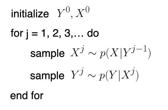
$x$와 $y$의 초기값을 정해주고 $p(x \mid y)$ 와 $p(y \mid x)$ 를 번갈아 가면서 sampling을 하면 burn-in period가 지나고 난 후에 초기값에 영향을 받지 않는 목표분포를 따르는 표본을 추출 할 수 있다. burn-in period에 대한 분석은 여기에 있다. 코드는 다음과 같다.

In [4]:

import random

def roll_a_die():
    # 주사위 눈은 1~6
    # 각 눈이 선택될 확률은 동일(uniform)
    return random.choice(range(1,7))

def direct_sample():
    d1 = roll_a_die()
    d2 = roll_a_die()
    return d1, d1+d2 # p(x,y)

def random_y_given_x(x):
    # x값을 알고 있다는 전제 하에 y값이 선택될 확률
    # y는 x+1, x+2, x+3, x+4, x+5, x+6 가운데 하나
    return x + roll_a_die()

def random_x_given_y(y):
    # y값을 알고 있다는 전제 하에 x값이 선택될 확률
    # 첫째 둘째 주사위 값의 합이 7이거나 7보다 작다면
    if y <= 7:
        # 첫번째 주사위의 눈은 1~6
        # 각 눈이 선택될 확률은 동일
        return random.randrange(1, y)
    # 만약 총합이 7보다 크다면
    else:
        # 첫번째 주사위의 눈은
        # y-6, y-5,..., 6
        # 각 눈이 선택될 확률은 동일
        return random.randrange(y-6, 7)
    
def gibbs_sample(num_iters=100):
    # 초기값이 무엇이든 상관없음
    x, y = 1, 2
    for _ in range(num_iters):
        x = random_x_given_y(y) # p(x|y)
        y = random_y_given_x(x) # p(y|x)
    return x, y # p(x,y) = p(x|y)p(y|x)

gibbs_sample 결과를 direct_sample(실제로는 알기 어려운 샘플)과 비교해보자.

샘플의 발생 빈도를 3차원 히스토그램으로 visualization 해볼 것이다.

In [5]:

n_samples = 1000
joint = np.array([direct_sample() for _ in range(n_samples)])
gibbs =  np.array([gibbs_sample() for _ in range(n_samples)])

fig, (ax1, ax2) = plt.subplots(nrows=1, ncols=2, figsize=(10, 4))
ax1 = fig.add_subplot(1,2,1, projection='3d')
hist1, xedges, yedges = np.histogram2d(joint[:,0], joint[:,1], normed=True,
                                      bins=[6,12], range=[[1, 7], [2, 13]])

xpos, ypos = np.meshgrid(xedges[:-1] + 0.25, yedges[:-1] + 0.25, indexing="ij")
xpos = xpos.ravel()
ypos = ypos.ravel()
zpos = 0

dx = dy = 0.5 * np.ones_like(zpos)
dz = hist1.ravel()

cmap = plt.cm.get_cmap('jet') # Get desired colormap - you can change this!
max_height = np.max(dz)   # get range of colorbars so we can normalize
min_height = np.min(dz)
# scale each z to [0,1], and get their rgb values
rgba = [cmap((k-min_height)/max_height) for k in dz] 

ax1.bar3d(xpos, ypos, zpos, dx, dy, dz, color=rgba, zsort='average',)
ax1.set_title("Real Samples")

ax2 = fig.add_subplot(1,2,2, projection='3d')
hist2, xedges, yedges = np.histogram2d(gibbs[:,0], gibbs[:,1], normed=True,
                                      bins=[6,12], range=[[1, 7], [2, 13]])

xpos, ypos = np.meshgrid(xedges[:-1] + 0.25, yedges[:-1] + 0.25, indexing="ij")
xpos = xpos.ravel()
ypos = ypos.ravel()
zpos = 0

dx = dy = 0.5 * np.ones_like(zpos)
dz = hist2.ravel()

cmap = plt.cm.get_cmap('jet') # Get desired colormap - you can change this!
max_height = np.max(dz)   # get range of colorbars so we can normalize
min_height = np.min(dz)
# scale each z to [0,1], and get their rgb values
rgba = [cmap((k-min_height)/max_height) for k in dz] 

ax2.bar3d(xpos, ypos, zpos, dx, dy, dz, color=rgba, zsort='average',)
ax2.set_title("Samples From Gibbs Sampling")

Text(0.5, 0.92, 'Samples From Gibbs Sampling')

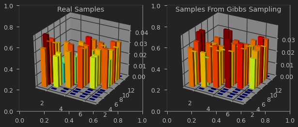
결합확률 분포가 얼마나 유사한가는 다음과 같은 KL divergence를 통해서 측정할 수 있다. \(\sum_{x,y} p(x,y) log \frac{p(x,y)}{q(x,y)}\)

KL divergence 값은 $0$과 $1$사이이며 $0$에 가까울 수록 비슷 하다는 뜻이다.

In [6]:

def kl_divergence(p, q, alpha=1e-8):
    return np.sum(np.where(p != 0, p * np.log((p + alpha) / (q + alpha)), 0))
kl_divergence(hist1, hist2)

0.029047606183849942

뽑을 샘플 수를 $N$ burn-in period를 $K$ 라고 하였을때 깁스 샘플링은 $O(KN)$이 걸린다.

In [7]:

n_samples = 1000

%timeit -r 3 -n 10 joint = np.array([direct_sample() for _ in range(n_samples)])
%timeit -r 3 -n 10 gibbs =  np.array([gibbs_sample() for _ in range(n_samples)])

1.67 ms ± 4.15 µs per loop (mean ± std. dev. of 3 runs, 10 loops each)
106 ms ± 492 µs per loop (mean ± std. dev. of 3 runs, 10 loops each)

또, 깁스 샘플링의 단점은 burn-in period 동안 state가 계속 바뀌는 데 그 바뀌는 값들을 버린다는 점과 언제까지 버려야하는 가에 대한 부분이 모호하다.

따라서, 이런 담점을 보완하는게 Metropolis Hastings의 motivation이다.

Metropolis Hastings

사전 지식: importance sampling

현재와 다음 스텝의 importance weight의 ratio를 acceptance rate으로 정의하여 샘플을 받아들일지 말지를 결정하는 알고리즘이다. \(A(x^{*} \mid x) = min(1, \frac{\frac{P(x^{*})}{Q(x^{*}\mid x)}} {\frac{P(x)}{Q(x \mid x^{*})}}) = min(1, \frac{P(x^{*}) Q(x\mid x^{*})} {P(x)Q(x^{*}\mid x)}) \\\)

• Initialize $x^{0}$
• Until Burn-in period:
  • Sample $x^{*} \sim Q(x^{*} \mid x)$
  • Sample $u \sim Uni(0,1) $
    • if $u < A(x^{*} \mid x) = min(1, \frac{P(x^{*}) Q(x \mid x^{*})} {P(x)Q(x^{*} \mid x)})$:
      • $x^{t} = x^{*}$ // transition
    • else:
      • $x^{t} = x$ // stay in current state

importance weight이 현재보다 커지면 accept하고 작아지면 그 비율만큼 accept 하면서 sample을 이동하다 보면 optimal point로 가게 된다.

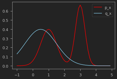
예제로 샘플링하기 어려운 실제 분포 $p_x$, 샘플링 하기 쉬운 분포 $q_x$를 가정하고, Metropolis Hastings를 구현해보자.

In [8]:

mu_target1 = 1
sigma_target1 = 0.5
mu_target2 = 3
sigma_target2 = 0.3

mu_proposal = 0.5
sigma_proposal = 1
p_x = lambda x: (stats.norm.pdf(x, loc=mu_target1, scale=sigma_target1) + \
            stats.norm.pdf(x, loc=mu_target2, scale=sigma_target2))/2  
q_xp_given_x = lambda xp, x: stats.norm.pdf(xp, x, sigma_proposal)

x = np.arange(-1,5,0.1)
plt.plot(x, p_x(x), label='p_x', color="red")
plt.plot(x, q_xp_given_x(x, mu_proposal), label='q_x', color="skyblue")
plt.legend()
plt.show()

In [9]:

N = 1000
samples = []  
x_t = 0.5
t = 0
while t < N:
    x_p = np.random.normal(x_t, sigma_proposal)  
    u = np.random.uniform(0, 1)  
    A = (p_x(x_p) * q_xp_given_x(x_t, x_p)) / (p_x(x_t) * q_xp_given_x(x_p, x_t) + 1e-6)
    if u <= A:  # accept        
        x_t = x_p
        samples.append(x_t)
        t += 1
        
samples = np.array(samples)

In [10]:

x = np.arange(-1,5,0.1)
plt.hist(samples, bins=x, density=True, color="skyblue", label="samples")
plt.plot(x, p_x(x), color="red", label='$p_x$')
plt.legend()

<matplotlib.legend.Legend at 0x7fa2dc5c35b0>

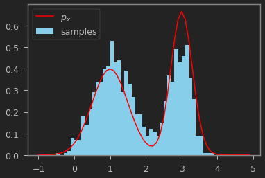
위의 결과를 보면 $p_x$를 잘 따르도록 샘플링 된 것을 알 수 있다.

GMM with Gibbs Sampling

이번에는 깁스샘플링을 활용하는 어플리케이션을 배워보자.

깁스 샘플링을 사용해서 가우시안 혼합 모델을 추정하는 문제를 풀어볼 것이다.

Metropolis Hastings을 적용하되 $i$ 번째 표본을 빼고 분포를 추정한다음 $i$번째 표본을 업데이트 해보자. gibbs sampling의 경우 $i$ 번째 sample을 제외한 상태에서 평가한 현시간과 다음시간의 importance weight에 대한 비율로 acceptance probability를 구한다. \(\require{cancel} \begin{align} A(x_{i}^{'}, x_{-i}\mid x_{i}, x_{-i}) &= min(1, \frac{\frac{P(x_{i}^{'} \mid x_{-i})}{Q(x_{i}^{'}, x_{-i}\mid x_{i}, x_{-i})} }{\frac{P(x_{i} \mid x_{-i})}{Q(x_{i}, x_{-i}\mid x_{i}^{'}, x_{-i})} }) \\ &= min(1, \frac{P(x_{i}^{'} \mid x_{-i}) Q(x_{i}, x_{-i}| x_{i}^{'}, x_{-i}) }{P(x_{i} \mid x_{-i}) Q(x_{i}^{'}, x_{-i}\mid x_{i}, x_{-i}) }) \\ &= min(1, \frac{P(x_{i}^{'} \mid x_{-i}) Q(x_{i}\mid x_{i}^{'}, x_{-i}) }{P(x_{i} \mid x_{-i}) Q(x_{i}^{'}| x_{i}, x_{-i}) }) \\ &= min(1, \frac{P(x_{i}^{'} \mid x_{-i}) Q(x_{i}\mid x_{-i}) }{P(x_{i} \mid x_{-i}) Q(x_{i}^{'}\mid x_{-i}) }) \;\; \mbox{$x_{i}$ and $x_{i}^{'}$ is independent } \\ &= min(1, \frac{\cancel{P(x_{i}^{'} \mid x_{-i})} \cancel{P(x_{i}| x_{-i})} }{\cancel{P(x_{i} \mid x_{-i})} \cancel{P(x_{i}^{'}\mid x_{-i})} }) \\ &= 1 \end{align}\) 놀랍게도 acceptance probabilty는 항상 $1$이 된다.
이를 이용하여 임의의 데이타 분포를 Multi-variate Guassian Mixture Distribution 으로 가정하고 acceptance probability를 항상 $1$로 보장하는 Gibbs Sampling를 사용해보자.
$x$ 는 데이타 point이고 $y$는 label 이라고 하자.

($i$는 샘플에 대한 index고, $k$는 class index)

• initialize variables $y_{i}$ for $i = 1, …, n$
• For $t = 1,..,T$:
  • For $i = 1,…,N$:
    • pick $i \in {1,…,n}$
    • For $k = 1,…,K$:
      • $p(y_{i} = k \mid x_{-i}, y_{-i}) \sim \mathcal{N}(x_{i} \mid \mu_{x_{-i},k}, \sigma_{x_{-i},k})$
    • update $y_{i} \leftarrow z_{i} \sim p(y_{i} \mid x_{-i}, y_{-i}) $

예제로 $x$는 $x_0 \sim \mathcal{N}(\mu_0, \sigma_0)$와 $x_1 \sim \mathcal{N}(\mu_1, \sigma_1)$ 의 혼합 분포라고 가정하였을 때, 이 분포를 추정해 볼 것이다.

우선 다음과 같이 $x$ 분포를 얻고, 원래 분포는 숨겨 놓는다.

In [11]:

fig, (ax0, ax1)  = plt.subplots(1,2)
ax0.axis('equal')
ax1.axis('equal')

n_sample = 300
mu0 = [1, 2]
sigma0 = np.eye(2) * np.sqrt(2)
x0 = np.random.multivariate_normal(mu0, sigma0, n_sample)
ax0.scatter(x0[:, 0], x0[:, 1], s = 10, alpha=0.5)

mu1 = [3, -3]
sigma1 = np.eye(2) * np.sqrt(3)
x1 = np.random.multivariate_normal(mu1, sigma1, n_sample)
ax0.scatter(x1[:, 0], x1[:, 1], s = 10, alpha=0.5)
ax0.scatter(*mu0, s=50, marker='*', color='b')
ax0.scatter(*mu1, s=50, marker='*', color='r')

x = np.concatenate([x0, x1])
ax1.scatter(x[:, 0], x[:, 1], s = 10, alpha=0.5)

<matplotlib.collections.PathCollection at 0x7fa2dc4e0670>

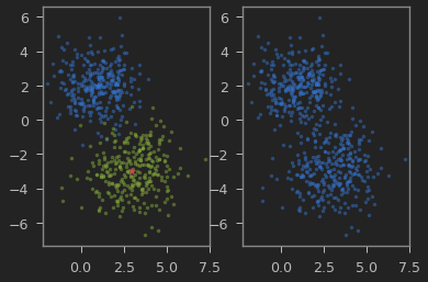
왼쪽그림에서 2가지 2차원 정균분포를 혼합해서 얻은게 오른쪽 그림에 보이는 $x$의 분포이다.

클래스의 갯수 K=2로 하여 iteration이 진행될 수록 본래의 분포를 찾아가는 과정을 볼 수 있다.

In [12]:

# intialize labels randomly
y = np.random.sample(size=len(x))
y[y > 0.5] = 1
y[y <= 0.5] = 0

# mu, sigma 초기화
mu0 = x[y==0].mean(axis=0)
sigma0 = np.diag(x[y==0].var(axis=0))
mu1= x[y==1].mean(axis=0)
sigma1 = np.diag(x[y==1].var(axis=0))

def visualize(x, y, mu0, sigma0, mu1, sigma1):
    plt.cla()
    plt.axis('equal')
    plt.title('{} iteration'.format(t))
    plt.scatter(*mu0, s=50, marker='*', color='skyblue')
    plt.text(*mu0, s='([{:.2f},{:.2f}], [{:.2f},{:.2f}])'.format(mu0[0], mu0[1],
                                                                sigma0[0][0], sigma0[1][1]))
    plt.scatter(*mu1, s=50, marker='*', color='red')
    plt.text(*mu1, s='([{:.2f},{:.2f}], [{:.2f},{:.2f}])'.format(mu1[0], mu1[1], 
                                                                sigma1[0][0], sigma1[1][1]))
    plt.scatter(x[y == 0][:,0], x[y == 0][:,1], s=10, alpha=0.5)
    plt.scatter(x[y == 1][:,0], x[y == 1][:,1], s=10, alpha=0.5)
    plt.show()


n_iter = 10
for t in range(n_iter):
    visualize(x, y, mu0, sigma0, mu1, sigma1)
    for i in range(len(x)):
#         i = random.sample(range(len(x)),1)[0]
        mu0= np.delete(x, i, axis=0)[np.delete(y, i, axis=0) == 0].mean(axis=0)
        cov0 = np.diag(np.delete(x, i, axis=0)[np.delete(y, i, axis=0) == 0].var(axis=0))
        y0 = mvn.pdf(x[i], mean=mu0, cov=cov0)
        mu1 = np.delete(x, i, axis=0)[np.delete(y, i, axis=0) == 1].mean(axis=0)
        cov1 = np.diag(np.delete(x, i, axis=0)[np.delete(y, i, axis=0) == 1].var(axis=0))
        y1 = mvn.pdf(x[i], mean=mu1, cov=cov1)
        y[i] = np.argmax([y0, y1])    

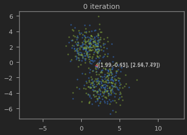
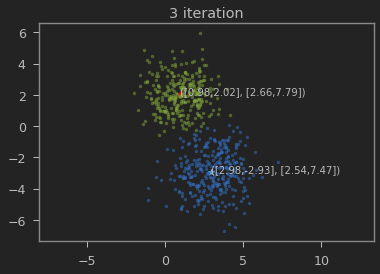
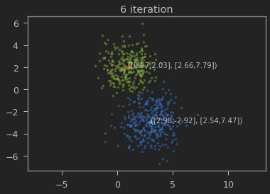
가우시안 혼합 모델이 1,2 와 3,-3에 가까운 값으로 추정되는 것을 볼 수 있다.
이곳에 들어가 보면 다양한 target 분포에 대해서 여러가지 알고리즘의 burn-in period가 될 때까지의 표본추출과정을 시각화하여 볼 수 있다.